Secondary Fund Economics Model
Private Equity Financial Model (Free Excel Download)
Evaluate secondary fund investments with entry discounts, portfolio liquidity, distributions, NAV changes, fees, and investor IRR, MOIC, and DPI outcomes.



professionals from Deloitte
Used by professionals from






About this model
Model secondary fund returns and J-curve for LP-view investors acquiring existing fund interests at a discount to reported NAV. The model projects cash inflows from distributions (15-30% of portfolio NAV realised annually in harvest phase) and outflows from unfunded commitment calls (10-30% of remaining unfunded per year). It calculates entry discount impact, models NAV appreciation/depreciation by fund vintage, and outputs gross and net IRR (before/after management fees and carry) plus DPI, RVPI, and TVPI multiples.
Key mechanics: purchase price is discounted NAV; distributions come in lumpy, back-loaded waves as underlying GP exits portfolio companies; unfunded calls must be reserved for; and the buyer assumes the GP's remaining hold period (typically 3-5 years of distributions). Leverage is optional (NAV facilities at 20-40% LTV with SOFR+200-400 bps). The model isolates gross returns (1.4-1.8x MOIC) from net-of-fee returns (1.3-1.6x) and includes sensitivity to entry discount and realisation pace.
Target audience: secondaries funds, pension funds, endowments, and institutional LPs evaluating secondary interest acquisitions. Critical for understanding tail-risk funds and how discount-to-NAV creates return potential at different realisation speeds.
What every model includes
Live formulas, no hardcoded values
Outputs are driven by live formulas, so the workbook updates from its assumptions instead of relying on hardcoded results.
All assumptions in one tab
Inputs are clearly marked in the Assumptions tab and separated from calculations, making it clear what to change and what to leave intact.
Statements always balancing
For integrated-statement models, the balance sheet, cash flow, and supporting schedules tie through properly.
Distinct schedules for clarity
Debt, working capital, taxes, and cash flow can get messy quickly. We group calculations in clear schedules, not across disconnected tabs.
No hidden macros or external links
There are no unexplained external workbook links or macros to undermine auditability or portability.
Changes flow through the model
Update a key driver and see the impact carry through the forecast, financing, and return outputs. We never use hardcoded numbers in formulas.
What's inside the Secondary Fund Economics Model
- Secondary position-level cash flow forecasts by vintage
- Portfolio composition by primary fund vintage and strategy
- Management fees, expense ratios, and carry impact
- J-curve modeling for fund maturity and return acceleration
- Weighted average IRR and MOIC by fund vintage
- LP cash distributions and reinvestment analysis
Secondary Fund Economics Model: How the Template Works
This secondary fund economics model evaluates a portfolio of secondary LP interests by tracking position-level cash flows, fees, and weighted IRR contributions. The template helps answer whether to invest and at what discount to NAV target returns are generated.
It moves beyond treating secondaries as a black box, offering a transparent LP-view framework for assessing the J-curve and return drivers.
Operating Drivers: Discount, Realisations, and Unfunded Calls
The model's core economic driver is the purchase price, calculated as reported NAV multiplied by one minus the entry discount. This discount determines the initial cost basis and, alongside realisation pace and NAV appreciation, shapes the return profile.
- Cash inflows come from distributions, modelled as a percentage of remaining NAV realised per period, with a minimum guard to prevent exceeding available value. Outflows include unfunded commitment calls, which reduce net returns if present.
- Transaction costs, ongoing management fees, and carried interest further affect net outcomes. The model explicitly separates gross and net figures, so users can see the impact of fee layers on returns.
These relationships capture the essential trade-offs in secondary investing.
Calculation Flow: From NAV Roll-Forward to Net Cash Flows
The calculation flow begins with the portfolio NAV roll-forward, which projects opening NAV, appreciation, realisations, write-downs, and closing NAV. This drives distribution timing and magnitude.
- The cash flow schedule combines the initial purchase price outflow, unfunded calls, distributions received, transaction costs, ongoing expenses, and any leverage draws or repayments. Net cash flow per period is then derived.
- To avoid circularity when leverage is used, repayments are based on prior-period distributions. The model also computes total invested capital as purchase price plus cumulative unfunded calls plus transaction costs.
This structured flow ensures that each component is explicitly linked, making the model auditable and consistent.
Key Outputs: IRR, MOIC, DPI, RVPI, and TVPI
The model produces a suite of return metrics: gross and net IRR, MOIC, DPI, RVPI, and TVPI. Gross MOIC uses cumulative distributions plus residual NAV to buyer, divided by total invested.
- DPI measures realised returns, while RVPI captures unrealised value. TVPI is simply the sum of DPI and RVPI.
- IRR is calculated from a cash flow stream that includes a negative Year 0 purchase price and subsequent net cash flows. Sensitivity tables allow users to examine how entry discount and realisation pace affect returns.
These outputs give a comprehensive view of both realised and unrealised performance, with clear separation between gross and net figures.
Practical Use: Validation and Sensitivity for Investment Decisions
The template includes validation checks to ensure model integrity: closing NAV and unfunded commitments stay non-negative, distributions do not exceed opening NAV, leverage respects the LTV cap, and TVPI equals DPI plus RVPI. These checks help catch common errors such as omitting unfunded calls or double-counting the purchase price.
- Sensitivity analysis on entry discount and realisation pace helps users understand how target returns vary under different assumptions. The model supports equity-funded deals and includes an optional leverage toggle, though leverage introduces circularity that is handled via prior-period distributions.
- By keeping the public download as a values-only preview, the template communicates the underlying structure without exposing live formulas. Users can assess whether a secondary portfolio meets return targets and at what discount.
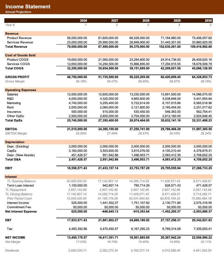
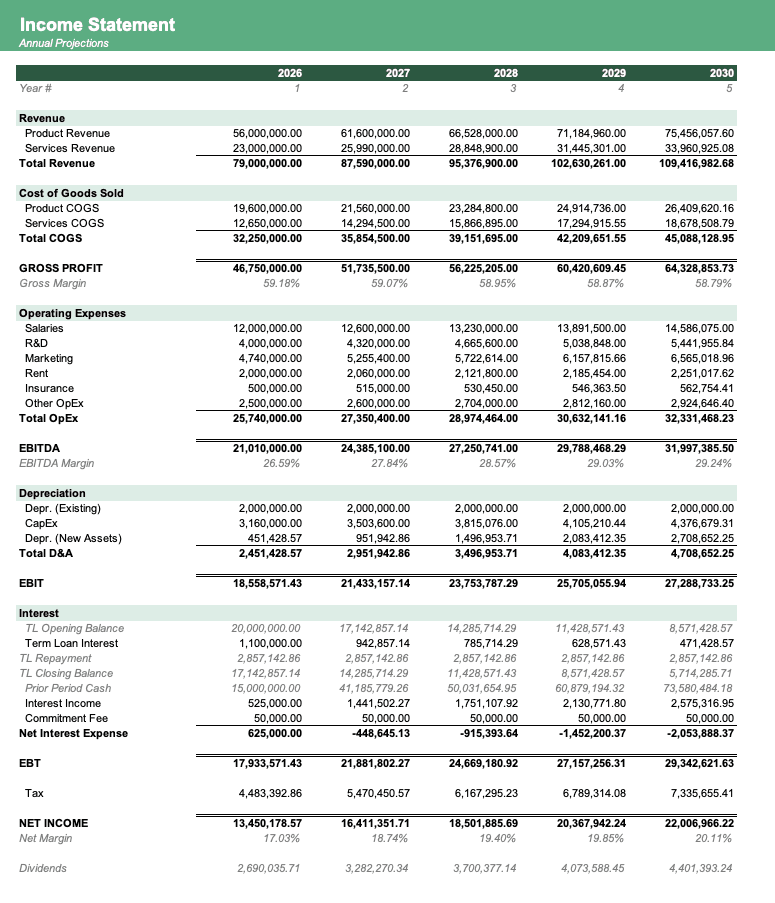
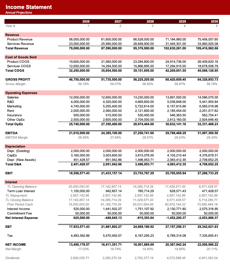
Formatted to IB standards
Named theme colors repaint the whole workbook in one click, on top of an investment-banking structure with clear input, output, and cross-sheet reference styling - brand-ready, institutional-grade, and fully auditable.

Created by ex-finance professionals
Hey, I’m Alex and I created Finamodel.
Over my years in the finance industry I kept building the same models over and over again. Same structure, same assumptions, different logo. So I started building frameworks to turn them into clean, reusable templates.
Every model here is one I’d actually use for a client, and I personally vet each one before it goes up.
I’m not an expert in every industry, but I’ve built enough models to know what belongs in one. And when something is completely foreign to me, I reach out to my network for experts to work on our models with us.
Having a template library on hand cuts a first build from hours to minutes.
Need help finding your model? You’ll find me in the Finamodel app!
Frequently asked
What is a secondary fund?+
A secondary fund buys existing LP interests in primary PE or VC funds, usually at a discount. LPs get quicker liquidity; the secondary manager gets an LP-like position with upside.
What is the J-curve in secondary funds?+
Early returns are negative or flat because of management fees and drag from positions purchased near the end of primary fund lives. Returns accelerate in years 3-5 as exits occur.
What is a typical secondary fund IRR?+
Secondary funds typically target 12-18% gross IRR depending on vintage and market. Net returns after fees typically range 10-15%.
How does vintage concentration affect risk?+
Heavy exposure to a single vintage year creates concentration risk if that vintage underperforms. The model shows vintage-level return contribution so you can identify this early.
Who uses secondary fund models?+
Fund of funds managers, pension funds, endowments, and LPs use them to evaluate secondary fund commitments, benchmark returns, and guide allocation decisions.
Have more financial modelling questions? Contact us
Related templates
Private Equity Fund Model
Fund-level cash flow, investment allocation, and LP returns including fees, distributions, and net IRR.
Fund of Funds Portfolio Model
Portfolio construction and performance tracking model for fund-of-funds vehicles investing across multiple manager-run funds.
Co-Investment Model
Track co-investor capital calls, distributions, and IRR by investor with waterfall mechanics.
Leveraged Buyout Model
Complete LBO analysis with debt financing structures, sponsor returns, and sensitivity to exit scenarios.