LBO Model Tutorial: Excel Guide

Key Takeaways
An LBO model projects equity returns by isolating the impact of leverage. Start with the sources and uses (where $600M comes from), build a five-year operating model, track debt paydown via a detailed debt schedule, and calculate IRR based on entry and exit valuations.
Debt paydown is the largest driver of equity returns in stable companies. If EBITDA grows 3-5% and you pay down $100M in debt, equity holders benefit from the combination of modest earnings growth plus leverage reduction. This is why PE firms focus on companies with stable, predictable cash flows.
Entry multiple matters more than exit multiple. Overpaying at acquisition (8.0x vs. 6.0x) is hard to overcome. Good deals are sourced at fair or modest entry multiples, with returns driven by debt paydown and operational improvement.
Build a debt schedule, not a black-box assumption. Explicitly model interest rates, amortization, and cash sweep. This forces you to understand the economics and exposes unrealistic assumptions.
Test sensitivity to entry and exit multiples. The returns table should show IRRs across a 2x2 grid of multiples, helping sponsors understand the deal's downside scenarios and covenant headroom.
Common pitfalls: forgetting stub-period interest, miscalculating interest on closing debt, not capping the cash sweep, ignoring covenants, confusing enterprise and equity value, and modeling impossible distributions. Each of these will distort returns by 200-500 bps.
A leveraged buyout (LBO) is the acquisition of a company using significant debt financing, with equity holders betting that operational growth and debt paydown will generate returns of 20-30% annually. Private equity firms use LBO models to underwrite deals, test sensitivity to different exit scenarios, and communicate investment theses to limited partners (LPs).
An LBO model is the most powerful financial modeling tool for PE investors because it isolates the impact of leverage on returns. Unlike a typical 3-statement financial model, which projects profit and loss, an LBO model forces three critical questions: How much debt can we safely use? How quickly must we pay it down? And what exit multiple do we need to hit our return targets?
The complete LBO model flow: from acquisition to exit.
This tutorial walks you through building an LBO model from scratch, with real numbers and every formula you need. We will model a $600M acquisition of a $100M EBITDA business and calculate the returns across different exit scenarios.
Transaction Structure: The Starting Point
An LBO begins with a transaction: the buyer (a PE fund) acquires a company from either the current owner or public shareholders. The purchase price is set as a multiple of EBITDA, the most standard valuation metric for corporate acquisitions.
Entry Multiple: The number of times EBITDA paid for the company. A 6.0x entry multiple means buying a $100M EBITDA business for $600M.
The $600M purchase price (called "Enterprise Value") is funded with a mix of debt and equity. The split determines the company's initial leverage and, crucially, the equity holders' return potential.
Capital Structure: Typical Debt vs. Equity Split
Unlike a real estate LBO, which may be 75-90% debt, corporate LBOs typically use 50-70% debt, with the remainder funded by equity from the PE fund. Here is a typical capital structure for a mid-market LBO:
| Financing Source | % of Purchase Price | Example ($600M Deal) |
|---|---|---|
| Senior Debt (Bank Loans) | 40% | $240M |
| Subordinated Debt (Mezz) | 10% | $60M |
| Equity (PE Fund) | 50% | $300M |
| Total | 100% | $600M |
This 60% debt / 40% equity split is conservative. Sponsors might push for 70% debt if the company has stable, predictable cash flows. The PE fund commits the $300M equity check upfront; the debt is borrowed from banks and other lenders and must be repaid from operating cash flow.
Sources and Uses: Where the Money Comes From and Goes
Every LBO starts with a sources and uses statement, a one-page summary showing where the $600M comes from (sources) and what it is used for (uses).
Sources = Uses. Always.
Worked Example: $600M Acquisition of $100M EBITDA Company
| SOURCES | USES | ||
|---|---|---|---|
| Senior Debt | $240.0M | Purchase Enterprise Value | $600.0M |
| Mezz Debt | $60.0M | Debt Issuance Costs | $10.0M |
| Equity | $300.0M | Transaction Fees | $2.0M |
| Total Uses | $612.0M | ||
| Total Sources | $600.0M |
Note: The numbers do not match because we have assumed $10M of debt issuance costs and $2M of transaction fees (investment banker, legal, accounting). These are funded from the initial equity check, increasing it from $300M to $312M. A real transaction might also include seller debt, holdback escrow, or assume existing liabilities.
For simplicity, our worked example will keep round numbers: $300M equity, $240M senior debt, $60M mezz debt, $600M enterprise value.
The Opening Balance Sheet
Once the transaction closes, we build the opening balance sheet. The target company's existing assets and liabilities are unchanged; we simply add the new debt and equity to the capital structure.
| Opening Balance Sheet | $M |
|---|---|
| ASSETS | |
| Working Capital | $40M |
| Fixed Assets (PP&E) | $160M |
| Total Assets | $200M |
| LIABILITIES & EQUITY | |
| Existing Liabilities | $60M |
| Senior Debt (New) | $240M |
| Mezz Debt (New) | $60M |
| Equity (PE Fund) | $300M |
| Less: Transaction Costs (Equity) | $(300M) |
| Total Liabilities & Equity | $360M |
Wait, this does not balance. The issue is that transaction costs (banker fees, legal) reduce the effective equity contributed. In practice, you would net them against the equity or assume they are paid separately. For this tutorial, assume they are absorbed by the sponsor and do not appear on the balance sheet.
The opening debt load is $300M ($240M senior + $60M mezz) on $100M EBITDA, or 3.0x Leverage. This is a moderate level; 4.0-5.0x is more aggressive.
Operating Model: Five Years of Growth
With the opening balance sheet set, we now project five years of operations. The operating model drives cash generation, which is then split between reinvestment (CapEx, working capital), debt repayment, and (eventually) equity proceeds.
Assumptions
For our $100M EBITDA business, assume the following five-year profile:
| Assumption | Value |
|---|---|
| Year 1 EBITDA | $100M |
| EBITDA Growth | 5% (Year 1), then 3% (Years 2-5) |
| EBITDA Margin | 20% of Revenue |
| Interest Rate (Senior Debt) | 6.0% |
| Interest Rate (Mezz Debt) | 9.0% |
| Tax Rate | 25% |
| CapEx as % of Revenue | 5% |
| Working Capital Change | 0% (assume no growth drag) |
Income Statement Projection
| Metric | Year 1 | Year 2 | Year 3 | Year 4 | Year 5 |
|---|---|---|---|---|---|
| EBITDA | $100.0M | $103.0M | $106.1M | $109.3M | $112.6M |
| EBITDA Margin | 20% | 20% | 20% | 20% | 20% |
| D&A | $(15.0M) | $(15.0M) | $(15.0M) | $(15.0M) | $(15.0M) |
| EBIT | $85.0M | $88.0M | $91.1M | $94.3M | $97.6M |
| Interest Expense | $(27.3M) | $(25.2M) | $(23.1M) | $(21.0M) | $(18.9M) |
| EBT | $57.7M | $62.8M | $68.0M | $73.3M | $78.7M |
| Taxes (25%) | $(14.4M) | $(15.7M) | $(17.0M) | $(18.3M) | $(19.7M) |
| Net Income | $43.3M | $47.1M | $51.0M | $55.0M | $59.0M |
Notice that even though EBITDA grows only 5% in Year 1 and 3% thereafter, net income grows faster (8-9%) because interest expense declines as debt is repaid. This is the power of leverage: operational growth is magnified by debt reduction.
Debt Schedule and Cash Sweep: Managing Leverage
The debt schedule is the heart of the LBO model. It tracks the opening debt balance, adds interest, subtracts mandatory amortization (if any), and then applies a cash sweep to use free cash flow for optional paydown.
Senior Debt: Typical Terms
Most senior bank debt in an LBO has the following structure:
| Parameter | Typical Value |
|---|---|
| Tenor | 5-7 years |
| Amortization | 1% per year (optional: more in later years) |
| Interest Rate | SOFR + 400-500 bps (6-7% all-in) |
| Financial Covenants | Maximum Leverage (e.g., Net Debt / EBITDA ≤ 4.0x) |
| Prepayment | 101-102% premium in Years 1-2, then 100% |
Mezz debt is more expensive (9-10% rates) but has looser amortization (often 0% until maturity) and fewer covenants.
Building the Debt Schedule
// Year 1 Senior Debt Calculation
// Opening Balance
Opening_Debt = 240

// Interest Expense (at 6% rate)
Interest = Opening_Debt * 0.06
// = 240 * 0.06 = 14.4M

// Mandatory Amortization (1% per year)
Mandatory_Amort = Opening_Debt * 0.01
// = 240 * 0.01 = 2.4M

// Closing Debt (before cash sweep)
Closing_Before_Sweep = Opening_Debt + Interest - Mandatory_Amort
// = 240 + 14.4 - 2.4 = 252M (if interest is accrued)

// In practice, interest is paid in cash, so:
Closing_Before_Sweep = Opening_Debt - Mandatory_Amort
// = 240 - 2.4 = 237.6M
Now we apply the cash sweep. Assume the business generates enough free cash flow (FCF) each year to pay down debt beyond the mandatory minimum. The sweep is calculated as:
// Free Cash Flow Available for Debt Repayment
FCF = Net_Income + D&A - CapEx - Change_in_WC

// For our example:
FCF_Year1 = 43.3 + 15.0 - 25.0 - 0 = 33.3M

// Cash Sweep: Assume 50% of FCF goes to debt (rest to sponsor)
Cash_Sweep = MIN(FCF * 0.5, Remaining_Debt_Before_Sweep)
// = MIN(33.3 * 0.5, 237.6) = MIN(16.65, 237.6) = 16.65M

// Closing Debt (after sweep)
Closing_Debt = Closing_Before_Sweep - Cash_Sweep
// = 237.6 - 16.65 = 220.95M
Full Five-Year Debt Schedule
| Year | Opening Debt | Interest (6%) | Mandatory Amort (1%) | Closing Before Sweep | Cash Sweep (50% FCF) | Closing Debt |
|---|---|---|---|---|---|---|
| 1 | $240.0M | $14.4M | $2.4M | $237.6M | $16.7M | $220.9M |
| 2 | $220.9M | $13.3M | $2.2M | $218.7M | $17.2M | $201.5M |
| 3 | $201.5M | $12.1M | $2.0M | $199.5M | $17.6M | $181.9M |
| 4 | $181.9M | $10.9M | $1.8M | $180.1M | $18.1M | $162.0M |
| 5 | $162.0M | $9.7M | $1.6M | $160.4M | $18.6M | $141.8M |
Notice that the closing debt in Year 5 is $141.8M, down from $240M at the start. This $98.2M debt reduction is critical to equity returns. The debt paydown comes from two sources: mandatory amortization and cash sweep (optional paydown). The cash sweep is the larger driver in this example, paying down $88M cumulatively over five years.
Mezz Debt: Simpler Structure
Mezz debt typically has 0% amortization and a bullet maturity at the end of the hold period. Its only change is interest accrual. For simplicity, assume it is paid off at exit:
| Year | Opening Balance | Closing Balance |
|---|---|---|
| 1-5 | $60.0M | $60.0M |
Exit Assumptions: The Terminal Value
After holding the company for five years, the sponsor sells it. The exit valuation is the foundation of equity returns. There are three common exit methods:
Exit Method 1: Multiple-Based (Most Common)
Vale the company at an "exit multiple" of EBITDA. If Year 5 EBITDA is $112.6M and we assume a 5.0x exit multiple:
Exit_EV = Year_5_EBITDA * Exit_Multiple
// = 112.6M * 5.0 = 563.0M
Note: The exit multiple is often lower than the entry multiple (6.0x entry vs. 5.0x exit) because the company has matured and growth is slowing. Sometimes, strong operational improvements justify a higher exit multiple.
Exit Method 2: LBO-Style (Less Common)
Some sponsors model the exit using a "dividend recapitalization," where they refinance the debt at a lower multiple and take a dividend. This is complex and rarely used in initial modeling.
Exit Method 3: IPO or Trade Sale
For high-growth companies, sponsors model an exit via IPO at a forward multiple (e.g., Year 6 EBITDA × 8.0x) or a trade sale to a larger company.
For this tutorial, we use Exit Method 1: 5.0x multiple on Year 5 EBITDA = $563.0M enterprise value.
Returns Calculation: IRR, MOIC, and Equity Multiple
With the operating model and debt schedule in place, we can now calculate returns to equity holders.
Waterfall from Enterprise Value to Equity Proceeds
The exit proceeds flow down as follows:
Enterprise Value (Exit)      = $563.0M
Less: Senior Debt            = $(141.8M)
Less: Mezz Debt              = $(60.0M)
Less: Preferred Equity       = $0
Equals: Common Equity Value  = $361.2M
The sponsor invested $300M in equity at closing. Exit proceeds of $361.2M on a $300M investment yield a simple multiple of 1.20x. But this does not account for the timing of the investment.
Internal Rate of Return (IRR)
The IRR accounts for timing. It is the discount rate that makes the net present value (NPV) of all equity cash flows equal to zero.
Equity Cash Flows:
| Year | Cash Flow | Description |
|---|---|---|
| 0 (Close) | $(300.0M) | Initial Equity Investment |
| 1-4 | $0 | No interim distributions |
| 5 | $361.2M | Exit Proceeds to Equity |
IRR Calculation:
=IRR(range_of_cash_flows)
// Cash flows: -300, 0, 0, 0, 0, 361.2
// Result: ~4.8% IRR
A 4.8% IRR is disappointing for a PE investment. This is because despite strong debt paydown, the exit multiple (5.0x) is lower than the entry multiple (6.0x), eroding returns. This illustrates a critical insight: leverage helps, but multiple compression kills returns.
Multiple on Invested Capital (MOIC)
MOIC is a simpler metric: total cash out / total cash in.
MOIC = Total Proceeds / Total Investment
// = 361.2 / 300 = 1.20x
A 1.20x MOIC over five years equates to roughly 4.8% IRR (they are linked, but MOIC ignores time value).
What If We Use a Higher Exit Multiple?
Now assume the company can be sold at 6.0x (same as entry multiple), rather than 5.0x:
Enterprise Value (6.0x Exit) = 112.6M * 6.0 = 675.6M
Less: Senior Debt            = $(141.8M)
Less: Mezz Debt              = $(60.0M)
Equity Proceeds              = $473.8M

MOIC = 473.8 / 300 = 1.58x
IRR  ≈ 9.8%
Still below target (20%+). The issue is that $100M EBITDA at 3% annual growth only reaches $112.6M in Year 5, which is a modest improvement. To hit a 20% IRR, the sponsor needs either faster EBITDA growth, a higher exit multiple, or lower entry leverage.
What If We Model the "Best Case"?
Assume the sponsor executes well: EBITDA grows 10% in Year 1 and 5% annually thereafter, reaching $127.6M in Year 5. Exit at 7.0x:
Enterprise Value (7.0x Exit) = 127.6M * 7.0 = 893.2M
Less: Senior Debt            = $(141.8M)
Less: Mezz Debt              = $(60.0M)
Equity Proceeds              = $691.4M

MOIC = 691.4 / 300 = 2.30x
IRR  ≈ 18.5%
This is closer to a PE target return, but still relies on optimistic execution (double-digit EBITDA growth + 700 bps multiple expansion).
Returns Sensitivity Analysis
The IRR and MOIC depend on two key levers: the entry multiple and the exit multiple. A sensitivity table shows how returns change across different combinations.
Exit Multiple × Entry Multiple Sensitivity Grid (5-Year Hold, $100M EBITDA, Base Case Growth)
| Entry Multiple | 4.0x Exit | 5.0x Exit | 6.0x Exit | 7.0x Exit | 8.0x Exit |
|---|---|---|---|---|---|
| 5.0x | 8.2% | 12.4% | 16.8% | 21.5% | 26.5% |
| 6.0x | 4.8% | 9.8% | 14.8% | 19.9% | 25.3% |
| 7.0x | 1.5% | 6.8% | 12.2% | 17.8% | 23.5% |
| 8.0x | (1.6%) | 3.9% | 9.6% | 15.5% | 21.7% |
Key observations:
- High Entry → Low Returns: Paying 8.0x entry EBITDA requires near-perfect execution (7-8x exit) to hit 20% IRRs. A $100M business at 8.0x costs $800M; leverage alone cannot save poor entry pricing.
- Flat Multiple (Entry = Exit) : Even with strong debt paydown, returns are mediocre (4.8% IRR at 6.0x × 6.0x). Sponsors need multiple expansion.
- Sweet Spot: Entry at 5.0x, exit at 6.0x or 7.0x, yields 16-21% IRRs. This is the "bread and butter" of PE deals.
Common Mistakes in LBO Modeling
Mistake 1: Forgetting to Accrue Interest on Closing Day
Interest does not wait until Year 1 end to accrue. If you close the deal on July 1, you immediately owe ~6 months of interest on the debt. Many modelers forget this, understating Year 1 interest and overstating Year 1 net income.
Fix: Add a "stub period" interest adjustment or pro-rate Year 1 interest based on the close date.
Mistake 2: Calculating Interest on Year-End Debt
Interest should be calculated on the average debt balance or the opening balance, not the closing balance (which already reflects repayments). Using closing balance overstates interest and understates returns.
// Wrong
Interest = Closing_Debt * Interest_Rate

// Right
Interest = Opening_Debt * Interest_Rate
// Or: Interest = AVERAGE(Opening_Debt, Closing_Debt) * Interest_Rate
Mistake 3: Modeling a Cash Sweep Without Limits
If the sweep exceeds remaining debt, you are trying to pay off debt that does not exist. The formula must include a MIN() function:
Cash_Sweep = MIN(Available_FCF, Remaining_Debt)
Mistake 4: Ignoring Debt Covenants
Bank debt is subject to financial covenants, such as "Maximum Leverage shall not exceed 4.0x." If your five-year projection violates the covenant, the deal breaches, and lenders can force a refinance or demand prepayment. Always check leverage against covenants in the sensitivity table.
Mistake 5: Confusing Enterprise Value with Equity Value
All multiples (entry, exit) apply to enterprise value, which is before deducting debt. Net of debt gives you equity value. A common error is to apply the exit multiple to "net income" instead of EBITDA, or to forget to subtract all debt categories (senior, mezz, preferred) before arriving at common equity.
Mistake 6: Modeling Distributions Without Funds Available
Some models assume the sponsor takes a dividend in Year 3 despite still holding significant debt. This is unrealistic and breaks covenant agreements. Never model interim distributions unless they are specifically endorsed by the debt agreement (e.g., dividend baskets).
Further Reading
For a deeper dive into DCF and valuation frameworks that complement LBO modeling, see our guide to DCF models in Excel. To understand the building blocks of any financial model, start with the 3-statement financial model. For a quick IRR calculation without manual Excel formulas, try our IRR calculator.

Alex Tapio
Founder of Finamodel • Professional Financial Modeller • Ex-Deloitte