Litigation Funding Portfolio
Private Equity Financial Model (Free Excel Download)
Forecast case costs, milestones, settlement probabilities, funding advances, recoveries, and investor waterfalls to evaluate litigation-finance portfolio returns.



professionals from Deloitte
Used by professionals from






About this model
A litigation-funding portfolio model captures the expected return of a closed-end fund that finances commercial-litigation, intellectual-property, antitrust, mass-tort, arbitration, and trade-secret cases in exchange for a contracted multiple of capital deployed on a win. The workbook runs across seven sheets - Cover, Assumptions, Case_Portfolio, Cashflows, Returns, Sensitivity, Checks - plus the shared Disclaimer. Every input is a named-range cell, every formula is one or two operations long, and the workbook passes static-value, self-reference, dead-assumption, and unused-named-range scans.
The case panel sits on the Assumptions sheet: eight cases with capital commitment, funding year (0-2), duration in years (2-4), base win probability (35-65%), MOIC on win (2.5-6.0x), and loss recovery rate (5-20% of capital). A Scenario_Sel parameter drives a CHOOSE() over three win-rate scalars (Base 1.00x, Bull 1.20x, Bear 0.75x), capped at 100% per case on the upside. The total committed capital is 37 million USD spread across eight diversified case types and three vintages - the sector convention for a sub-$50M emerging-manager fund.
The Case_Portfolio sheet computes per-case expected value: EV recovery = Capital × (Adjusted Win × MOIC + (1 − Adjusted Win) × Loss Recovery), then EV profit, EV / cost ratio, and resolution year (funding year + duration). The Cashflows sheet rolls annual portfolio cashflows - per-case capital out triggered by funding year, per-case expected recoveries triggered by resolution year, plus a 2% management fee drag every year on committed capital - into net pre-carry and cumulative pre-carry rows.
Carry is computed European-style: only in the terminal year, only on profits above the hurdle × weighted-average duration, at 20% of the excess. This matches institutional fund convention for closed-end vehicles. The Returns sheet headlines gross IRR (23%), gross MOIC (2.0x), net IRR (21%), net MOIC (1.7x), TVPI, DPI, and portfolio NPV at a 12% discount rate, plus the capital-weighted win rate, weighted-average duration, total capital deployed, expected recovery, expected profit, and cumulative fees and carry paid.
The Sensitivity sheet runs a 5x5 grid of net IRR across win-rate scalars (0.6x to 1.4x) and MOIC multipliers (0.8x to 1.2x) using a closed-form approximation that lands within tolerance of the headline IRR at the centre cell. The Checks sheet runs seven cross-sheet validations - capital deployed equals commitment, all adjusted win probabilities ≤ 100%, every case EV recovery non-negative, carry confined to the final period, carry respects the hurdle gate, net MOIC ≤ gross MOIC, and the sensitivity centre cell within tolerance of the headline net IRR.
Target users are litigation-finance LPs (pension funds, family offices, alternative-asset allocators), fund GPs raising or reporting on a litigation-finance vehicle, and bankers underwriting LP commitments. The model is calibrated against published gross returns from Burford Capital, Omni Bridgeway, Therium, and Parabellum - typical commercial-litigation funds report 20-35% gross IRR and 15-25% net IRR on 2.5-3.5 year duration. Use the scenario selector for win-rate stress testing, edit the case panel for portfolio diversification analysis, and flex the fee-and-carry inputs to compare the LP cost of 2-and-20 against alternative structures.
What every model includes
Live formulas, no hardcoded values
Outputs are driven by live formulas, so the workbook updates from its assumptions instead of relying on hardcoded results.
All assumptions in one tab
Inputs are clearly marked in the Assumptions tab and separated from calculations, making it clear what to change and what to leave intact.
Statements always balancing
For integrated-statement models, the balance sheet, cash flow, and supporting schedules tie through properly.
Distinct schedules for clarity
Debt, working capital, taxes, and cash flow can get messy quickly. We group calculations in clear schedules, not across disconnected tabs.
No hidden macros or external links
There are no unexplained external workbook links or macros to undermine auditability or portability.
Changes flow through the model
Update a key driver and see the impact carry through the forecast, financing, and return outputs. We never use hardcoded numbers in formulas.
What's inside the Litigation Funding Portfolio
- 8-case commercial-litigation panel with capital, funding year, duration, win prob, MOIC on win, loss recovery
- Scenario selector (Base 1.00x, Bull 1.20x, Bear 0.75x) driving win-rate scalars across the panel via CHOOSE()
- Case_Portfolio sheet with adjusted win probability, EV recovery, EV profit, EV/cost ratio, resolution year
- Cashflows sheet with per-case capital out by funding year and recovery by resolution year, plus mgmt fee, carry, net pre and post
- European-style waterfall: 2% mgmt fee on commitment, 20% carry on profits above 8% hurdle by weighted-avg duration
- Returns sheet with Gross IRR / MOIC, Net IRR / MOIC, TVPI, DPI, NPV at 12%, and portfolio composition
- 5x5 Sensitivity grid: win-rate scalar (0.6x-1.4x) by MOIC multiplier (0.8x-1.2x) producing closed-form Net IRR
- Seven validation checks: deployed equals commitment, win prob bounded, EV non-negative, carry mechanics, sensitivity centre matches headline
Litigation Funding Portfolio: How the Fund Model Works
This litigation funding template shows how an eight-case commercial litigation finance portfolio is evaluated from the investor side over a six-year horizon. It combines per-case expected value with portfolio cashflows, an illustrative 2-and-20 fee structure, gross and net return metrics, and a sensitivity grid on win rates and contracted multiples.
How the Case Portfolio Is Built
The portfolio contains eight commercial litigation cases representing breach of contract, intellectual property, antitrust, mass tort, international arbitration, securities, trade secret, and construction lien matters. Total committed capital is spread across funding years zero to two, with individual case durations of two to four years, so capital deploys gradually and resolutions cluster in later years.
- Each case carries a capital commitment, a base win probability, a contracted multiple on a win, and a loss recovery assumption. Loss recovery is an input for partial settlement proceeds on unsuccessful cases.
- This construction diversifies the fund across case type and timeline rather than concentrating exposure in one dispute.
Per-Case Expected Value Logic
Expected value is calculated case by case before any portfolio aggregation. A scenario selector applies a win-rate scalar to every case's base win probability, capped at one hundred percent on the upside.
- Adjusted probability then blends the contracted multiple on a win with the loss recovery on a loss, weighted by those probabilities. Subtracting capital gives expected profit, and dividing expected recovery by capital gives the expected recovery-to-capital ratio.
- Each case's resolution year is its funding year plus duration. Because the same scalar moves every case, the scenario layer shifts portfolio-level outcomes without changing the underlying case assumptions.
Portfolio Cashflows and Fee Waterfall
Year-by-year cashflows combine capital outflows, expected recoveries, management fees, and carried interest. Management fees are charged on committed rather than deployed capital at a constant annual rate.
- Carry is calculated only in the terminal year on profits above the input preferred return scaled by weighted-average duration, following a European-style, portfolio-level waterfall. Each year's net cashflow feeds a cumulative pre-carry balance used to test the hurdle.
- Fees and carry are deducted from gross cash flows to calculate LP net cash flows. The model includes a check comparing gross and net return multiples.
Returns, Sensitivity, and Practical Use
Outputs include gross and net IRR, MOIC, TVPI, DPI, portfolio NPV at the input discount rate, and weighted-average duration and win rate.
- A five-by-five sensitivity grid varies the win-rate scalar and contracted multiples, approximating net IRR across win-rate and MOIC bands.
- The grid is a closed-form simplification that does not reproduce full deployment timing and can be compared with the headline result at the centre cell.
- Practically, the model lets an evaluator see how case mix, win-rate assumptions, and multiple haircuts interact with the fee structure, and understand which drivers matter most for LP outcomes.
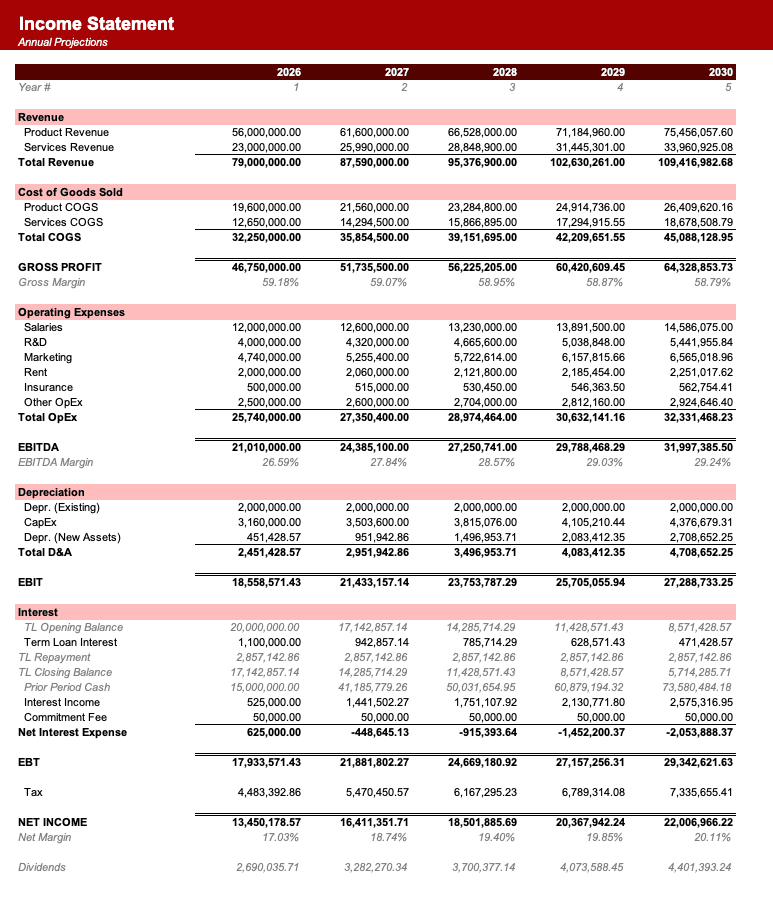
Formatted to IB standards
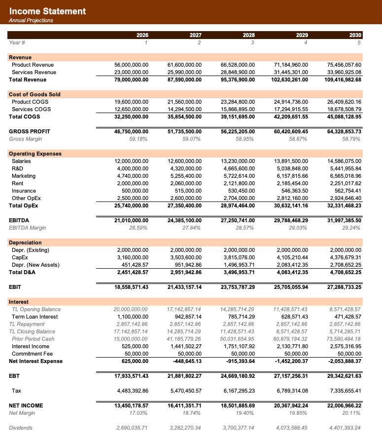
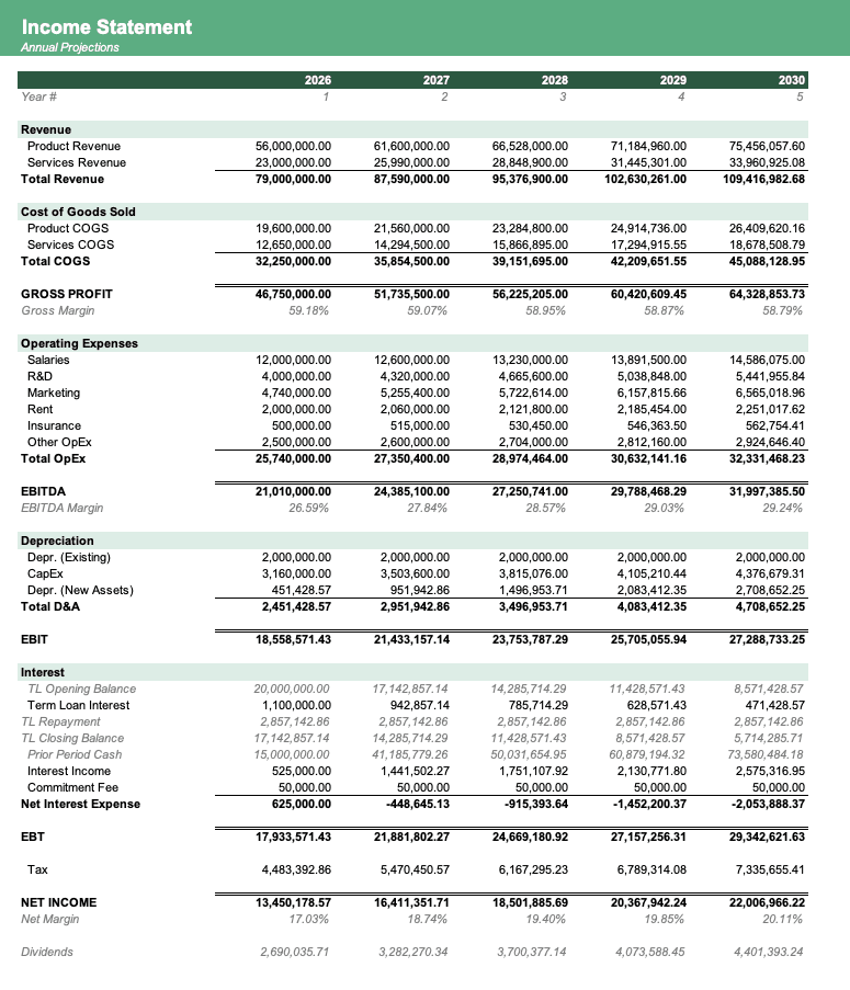
Named theme colors repaint the whole workbook in one click, on top of an investment-banking structure with clear input, output, and cross-sheet reference styling - brand-ready, institutional-grade, and fully auditable.

Created by ex-finance professionals
Hey, I’m Alex and I created Finamodel.
Over my years in the finance industry I kept building the same models over and over again. Same structure, same assumptions, different logo. So I started building frameworks to turn them into clean, reusable templates.
Every model here is one I’d actually use for a client, and I personally vet each one before it goes up.
I’m not an expert in every industry, but I’ve built enough models to know what belongs in one. And when something is completely foreign to me, I reach out to my network for experts to work on our models with us.
Having a template library on hand cuts a first build from hours to minutes.
Need help finding your model? You’ll find me in the Finamodel app!
Frequently asked
What is a litigation-funding model?+
A litigation-funding model captures the expected return of a closed-end fund that finances commercial-litigation, IP, antitrust, mass-tort, and arbitration cases in exchange for a contracted multiple of capital on a win. It is how institutional LPs underwrite whether a diversified case panel and the 2-and-20 fee structure clears the required net IRR hurdle.
How does the expected-value formula handle losing cases?+
Each case has a Win Prob and a Loss Recovery rate. EV recovery = Capital times (Adjusted Win times MOIC plus (1 minus Adjusted Win) times Loss Recovery). Loss recovery captures partial settlements on losing cases - typical 5 to 20% of capital - because defendants often settle to avoid retrial risk and legal-cost reimbursement claims.
What does the scenario selector do?+
Scenario_Sel (1=Base, 2=Bull, 3=Bear) runs a CHOOSE() over three win-rate scalars (1.00x, 1.20x, 0.75x). The selected scalar multiplies every case base win probability, capped at 100%. Flipping the cell on Assumptions recomputes the entire portfolio in one keystroke - Case_Portfolio, Cashflows, Returns, Sensitivity, and Checks all follow.
Why is carry only paid in the terminal year?+
The model uses a European-style waterfall - carry is calculated portfolio-level after all capital is returned plus the preferred return (8% times weighted-avg duration). This is the institutional LP convention for closed-end fund vehicles. Deal-by-deal carry would fire on each case settlement, which favours the GP at the LP expense.
Can I model insurance-wrapped litigation finance?+
Not directly. This template models a fully-funded fund with no ATE (After-The-Event) insurance or capital-protected note structure. To layer insurance, add a premium row (cost) and a recovery floor (proceeds) per case on Assumptions, then adjust the loss-recovery formula to take MAX(LossRec, Insurance_Floor). The fee and carry mechanics stay unchanged.
Have more financial modelling questions? Contact us
Related templates
Direct Lending Fund Model
Financial model for direct lending fund with loan origination, yield, losses, and fund returns.
Distressed Debt Analysis
Valuation and recovery analysis for distressed bonds and loans with recovery timeline and outcomes.
Private Equity Fund Model
Fund-level cash flow, investment allocation, and LP returns including fees, distributions, and net IRR.
Leveraged Buyout Model
Complete LBO analysis with debt financing structures, sponsor returns, and sensitivity to exit scenarios.