Monte Carlo Simulation in Excel: A Step-by-Step Guide
Key Takeaways
- Monte Carlo turns one number into a distribution. Instead of a single profit estimate, you get a mean, a spread, percentiles, and the probability of specific outcomes such as a loss.
- You do not need an add-in. Native Excel -
RAND(),NORM.INV, a one-variable Data Table, and summary functions likePERCENTILE.INCandCOUNTIF- is enough to build a complete Monte Carlo simulation in Excel. - Choose distributions deliberately. Normal for symmetric inputs, Uniform when you only know the bounds, Triangular for min/most-likely/max estimates, Lognormal for non-negative skewed quantities.
- The mean confirms; the tails inform. For independent inputs the simulated mean lands on your base case. The value Monte Carlo adds is everything around the mean - the P10, the P90, and the probability of loss.
- 10,000 trials is the practical sweet spot. Precision improves with the square root of the trial count, so quadruple the trials to halve the error. Freeze the results with Paste Values before reporting.
- Watch for correlation and wrong distributions. The two mistakes that most distort real Monte Carlo models are treating correlated inputs as independent and defaulting to Normal for everything.
Monte Carlo simulation is the honest way to model an uncertain future: it stops you pretending you know the one number, and forces you to reckon with the range. Pair it with structured scenario planning for a complete picture of upside, base, and downside - one gives you the hand-picked cases, the other the full probability weather map.
A Monte Carlo simulation in Excel replaces a single-point forecast with thousands of randomized trials, turning uncertain inputs into a full probability distribution of outcomes. Instead of asking "what is the profit?" you ask "what is the range of profit, and how likely is a loss?" This guide shows you how to build a Monte Carlo simulation in Excel from scratch - using only native functions like RAND and NORM.INV plus a Data Table - with a fully worked example, the exact formulas, and the summary statistics that make the results decision-ready.
Every forecast is wrong. The question is by how much, and in which direction. A traditional model gives you one number - a base-case NPV, a projected profit, a target valuation - built on point estimates for every input. But your inputs are not certain: units sold, unit cost, growth rate, and discount rate are all ranges, not fixed values. A Monte Carlo simulation embraces that uncertainty directly. It assigns a probability distribution to each risky input, draws a random value from each one, recalculates the model, and repeats the process thousands of times. The result is not a single answer but a distribution: a mean, a spread, percentiles, and - most usefully - the probability of an outcome you care about, such as a loss.
The best part: you do not need a paid add-in like @RISK or Crystal Ball to do this. Native Excel has everything you need. This tutorial builds a complete Monte Carlo simulation in Excel step by step.
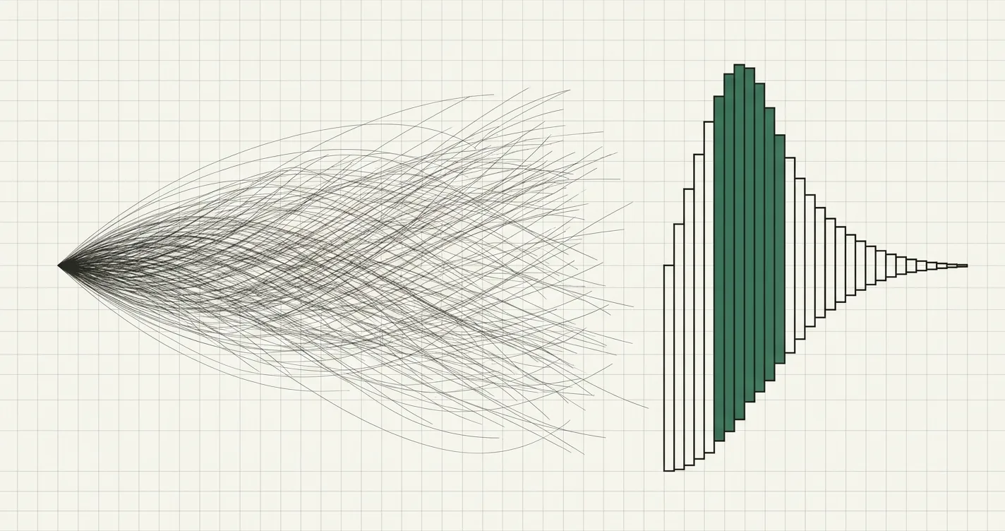
The Monte Carlo loop: from uncertain inputs to a full distribution of outcomes.
What a Monte Carlo Simulation Actually Does
The name comes from the casino district in Monaco - the method relies on repeated random sampling, the same way a gambler faces repeated random draws. In a financial model, the idea is simple:
- Pick the output you want to understand (profit, NPV, IRR, ending cash).
- For each uncertain input, choose a probability distribution that describes the range of plausible values (normal, uniform, triangular, and so on).
- Run one trial: draw a random value from each input's distribution and calculate the resulting output.
- Run thousands of trials, each with a fresh set of random draws.
- Analyse the collection of outputs as a distribution - its average, its spread, and the probability of specific outcomes.
Where a single-point model tells you the profit will be $50,000, a Monte Carlo simulation tells you the expected profit is around $50,000, but the realistic range spans from a $23,000 loss to a $123,000 gain, and there is roughly a one-in-five chance the project loses money altogether. That is a far more honest - and more useful - answer.
This is also what separates Monte Carlo from its simpler cousins. Sensitivity analysis flexes one input at a time; scenario analysis tests a handful of hand-picked combinations (base, bull, bear). Monte Carlo tests thousands of combinations simultaneously and weights them by how likely each is. If you are new to the simpler techniques, read our guide to sensitivity analysis in Excel first - Monte Carlo is the natural next step up.
The Building Blocks: Excel's Random Functions
Everything starts with RAND(), which returns a uniformly distributed random number between 0 (inclusive) and 1 (exclusive). On its own it is not very useful, but combined with inverse-distribution functions it can generate a draw from almost any distribution.
The key trick is inverse transform sampling: feed a uniform random number from RAND() into the inverse cumulative distribution function of the distribution you want. Excel has these built in.
Normal distribution
The workhorse. Use it for inputs that cluster symmetrically around a mean - revenue, costs, growth rates.
// Random draw from a Normal distribution with a given mean and standard deviation
= NORM.INV(RAND(), mean, standard_deviation)

// Example: units sold, mean 10,000, standard deviation 2,000
= NORM.INV(RAND(), 10000, 2000)
Uniform distribution
Every value in a range is equally likely. Good when you only know the bounds, not the shape.
// Continuous uniform between a lower bound a and upper bound b
= a + RAND() * (b - a)

// Example: discount rate equally likely to be anywhere from 8% to 12%
= 0.08 + RAND() * (0.12 - 0.08)
For a whole-number uniform draw (e.g., a random integer between 1 and 6), use =RANDBETWEEN(1, 6).
Triangular distribution
The favourite of practitioners who think in "min / most-likely / max" terms - it needs only three estimates and no statistics background. Its mean is simply (min + mode + max) / 3. The formula is longer because it stitches two curves together at the mode:
// First, put ONE random draw in a helper cell, say U1:
U1: = RAND()

// Then reference that single U1 in the triangular formula
// a = min, c = mode, b = max
= IF( U1 < (c - a) / (b - a),
      a + SQRT( U1 * (b - a) * (c - a) ),
      b - SQRT( (1 - U1) * (b - a) * (b - c) ) )
Critical detail: notice the formula reuses the same helper cell U1 in both branches. A common beginner error is to call RAND() multiple times inside one formula - each call returns a different number, which corrupts the sampling. Always draw the random number once, store it, then reference it.
Lognormal distribution
For quantities that cannot go negative and are right-skewed (asset prices, project durations):
= LOGNORM.INV(RAND(), mean_of_ln, sd_of_ln)
Worked Example: Will This Product Launch Make Money?
Let us build a real simulation. A company is evaluating a one-year product launch. The profit equation is straightforward:
Profit = Units Sold x (Price - Unit Cost) - Fixed Costs
Two of these inputs are uncertain. Here are the assumptions:
| Input | Type | Estimate |
|---|---|---|
| Units Sold | Uncertain (Normal) | mean 10,000, std dev 2,000 |
| Price | Fixed | $50 |
| Unit Cost | Uncertain (Normal) | mean $30, std dev $4 |
| Fixed Costs | Fixed | $150,000 |
The single-point answer (and why it misleads)
If you plug in the mean of every input, you get the deterministic base case:
Profit = 10,000 x ($50 - $30) - $150,000
       = 10,000 x $20 - $150,000
       = $200,000 - $150,000
       = $50,000
A $50,000 profit looks comfortable. But that number hides all the risk. What happens in a bad year where volume disappoints and costs run high at the same time? The single-point model cannot tell you. Monte Carlo can.
Setting up one trial in Excel
Lay out the model so each uncertain input is a formula, and the output references them:
// Cell B2 - Units Sold (random each recalculation)
= NORM.INV(RAND(), 10000, 2000)

// Cell B3 - Unit Cost (random each recalculation)
= NORM.INV(RAND(), 30, 4)

// Cell B4 - Profit for this trial
= B2 * (50 - B3) - 150000
Every time Excel recalculates (press F9), cells B2 and B3 draw fresh random values and B4 shows the profit for that single trial. Here are three trials I captured by hand so you can verify the arithmetic:
| Trial | Units Drawn | Unit Cost Drawn | Contribution Margin | Profit |
|---|---|---|---|---|
| 1 | 8,500 | $33 | $17 | 8,500 x 17 - 150,000 = -$5,500 |
| 2 | 11,200 | $28 | $22 | 11,200 x 22 - 150,000 = $96,400 |
| 3 | 9,800 | $31 | $19 | 9,800 x 19 - 150,000 = $36,200 |
Notice Trial 1: a below-average volume combined with an above-average cost produces an outright loss of $5,500 - exactly the downside the single-point model concealed. One trial tells you nothing on its own. The power comes from running thousands.
Running Thousands of Trials with a Data Table
The elegant native-Excel technique for repeating a calculation many times is a one-variable Data Table. Here is the setup:
- In column A, list your trial numbers:
1, 2, 3, ... 10000down cells A2:A10001. - In the cell one row up and one column right of the first trial number - cell B1 - put a formula that simply references your output:
=B4(the Profit cell). This is the "output to capture." - Select the whole block A1:B10001.
- Go to Data -> What-If Analysis -> Data Table.
- Leave Row input cell blank. For Column input cell, point to any empty cell that your model does not use - for example
$D$1. - Click OK.
Excel now recalculates the entire model once for each of the 10,000 rows, and because RAND() is volatile it produces a fresh random draw every time. Column B fills with 10,000 independent profit outcomes - your simulated distribution.
// B1 - the cell the Data Table captures for every trial
= B4

// Column input cell in the Data Table dialog: any unused cell
$D$1
Tip: if the sheet becomes slow, switch calculation to Automatic Except for Data Tables (Formulas -> Calculation Options), then press F9 to re-run the whole simulation on demand.
Reading the Results: From 10,000 Numbers to a Decision
Ten thousand raw numbers are useless until you summarise them. These are the formulas that turn the trial column (call the range Results) into an answer:
// Expected (mean) profit
= AVERAGE(Results)

// Spread of outcomes
= STDEV.S(Results)

// Downside case - 10th percentile
= PERCENTILE.INC(Results, 0.10)

// Median - 50th percentile
= PERCENTILE.INC(Results, 0.50)

// Upside case - 90th percentile
= PERCENTILE.INC(Results, 0.90)

// Probability the project loses money
= COUNTIF(Results, "<0") / COUNT(Results)
Running the simulation on our product-launch model produces results like the following (your exact figures will shift slightly on every recalculation - that is the nature of random sampling):
| Statistic | Value | What it tells you |
|---|---|---|
| Mean profit | ~$50,000 | Matches the single-point base case - as it should |
| Standard deviation | ~$57,000 | The outcomes are very spread out relative to the mean |
| 10th percentile (P10) | ~-$23,000 | A bad-but-plausible year loses ~$23k |
| 50th percentile (P50) | ~$50,000 | The median outcome |
| 90th percentile (P90) | ~$123,000 | A good year clears ~$123k |
| Probability of loss | ~19% | Roughly a one-in-five chance of losing money |
This is the payoff. The mean confirms the base case, but the simulation reveals what the base case hid: the outcomes swing across a $146,000 band from P10 to P90, and there is a ~19% chance the launch loses money. A CFO deciding whether to green-light this launch now has a risk profile, not just a hopeful point estimate.
Why the mean equals the base case
It is not a coincidence that the simulated mean (~$50,000) lands on the deterministic base case. When your uncertain inputs are independent and enter the model without being multiplied together in a skewing way, the average of many trials converges on the result you get from plugging in the average of each input. Monte Carlo does not change your expected answer - it reveals the distribution around it.
Visualising the distribution
Group the 10,000 outcomes into bins with FREQUENCY and chart them as a column histogram. An illustrative shape looks like this:
| Profit Range | Approx. Trials (of 10,000) | Share |
|---|---|---|
| Below -$50,000 | 400 | 4% |
| -$50,000 to $0 | 1,500 | 15% |
| $0 to $50,000 | 3,100 | 31% |
| $50,000 to $100,000 | 3,100 | 31% |
| $100,000 to $150,000 | 1,500 | 15% |
| Above $150,000 | 400 | 4% |
The two loss buckets (below $0) sum to 1,900 trials - 19% - which ties out with the probability-of-loss formula above. In a real run the right tail is slightly longer than the left (a mild positive skew), because profit is bounded below by the fixed cost but has no ceiling on the upside.
How Many Trials Do You Need?
More trials produce a more stable estimate, but with diminishing returns. The precision of the simulated mean is governed by the standard error:
Standard Error of the Mean = Standard Deviation / SQRT(Number of Trials)
For our model, with a standard deviation of about $57,000:
| Trials | Standard Error of the Mean | Interpretation |
|---|---|---|
| 1,000 | 57,000 / SQRT(1,000) = ~$1,803 | Mean is accurate to roughly +/- $1,800 |
| 10,000 | 57,000 / SQRT(10,000) = ~$570 | Mean is accurate to roughly +/- $570 |
| 100,000 | 57,000 / SQRT(100,000) = ~$180 | Mean is accurate to roughly +/- $180 |
Notice the pattern: to cut the error in half you must quadruple the trials (because of the square root). For most business decisions, 10,000 trials is the sweet spot - precise enough to trust the percentiles, fast enough to recalculate in a second or two. Use 1,000 for a quick look and reserve 100,000 for cases where you need tight tail estimates.
Freezing Your Results
Because RAND() is volatile, every edit, save, or F9 keypress re-randomises the entire simulation - your numbers move every time. When you are ready to report a specific run:
- Select the results column.
- Copy it.
- Paste as Values (Paste Special -> Values) over itself.
The numbers are now frozen static values, safe to chart and share. Keep the live formula version on a separate tab if you want to re-run later. This "snapshot then report" workflow is the single most common thing beginners forget, and it is why two people looking at the same file sometimes see different numbers.
Common Mistakes to Avoid
- Calling RAND() multiple times in one formula. Each
RAND()is an independent draw. If your triangular or custom-distribution formula referencesRAND()twice, the two branches use different random numbers and the sampling is wrong. Draw once into a helper cell, then reference it. - Ignoring correlation between inputs. Real inputs are often linked - high sales volume may coincide with higher unit costs (capacity strain) or lower ones (economies of scale). Treating everything as independent when it is not can badly understate or overstate risk. For correlated inputs you need a correlation technique (Cholesky decomposition) rather than naive independent draws.
- Using the wrong distribution. Defaulting to Normal for everything is convenient but wrong when a quantity cannot go negative (use Lognormal) or when you only have min/most-likely/max estimates (use Triangular). A Normal distribution for "units sold" can technically produce negative units - cap it with
MAX(0, ...)if that matters. - Too few trials. Reading percentiles off a 100-trial run gives noisy, unreliable tail estimates. Use at least 1,000; prefer 10,000.
- Reporting a live (unfrozen) run. Screenshotting results while
RAND()is still volatile means the numbers changed the instant you pressed a key. Freeze with Paste Values before reporting. - Confusing the mean with the outcome. The expected value is not what will actually happen - it is the long-run average of many parallel universes. The whole point of Monte Carlo is the spread and the probability of bad outcomes, not the single mean number.
- Forgetting to sanity-check. If your simulated mean does not roughly match your deterministic base case (for independent inputs), something is wired wrong. Always reconcile the two before trusting the distribution.

Alex Tapio
Founder of Finamodel • Professional Financial Modeller • Ex-Deloitte