Terminal Value: Gordon Growth vs Exit Multiple
Key Takeaways
- Terminal value usually drives the valuation. It is commonly 60-80% of enterprise value, so it deserves more scrutiny than the explicit forecast, not less.
- Two methods, one discipline. Gordon Growth (perpetuity) is intrinsic and best for mature companies; the exit multiple is market-based and useful with strong comparables. Calculate both.
- The formula: TV = FCF_final x (1 + g) / (WACC - g) for Gordon Growth; TV = EBITDA_final x exit multiple for the multiple method. Discount either back by (1 + WACC) ^ N.
- Always cross-check. Back out the implied exit multiple from your Gordon Growth TV, and the implied perpetuity growth from your exit-multiple TV. Both should land in sensible ranges.
- Respect the ceilings. Terminal growth must stay below long-run GDP growth (2-3%) and strictly below WACC. Exit multiples should reflect mature, terminal-year peers.
- Normalise the final year. The perpetuity inherits whatever is in your last forecast year forever - so strip out one-offs and bring CapEx, working capital, and margins to steady state first.
- Show a range. Pair both methods with a WACC-vs-growth sensitivity table and present the valuation as a band, never a single point.
Terminal value is where most DCFs are won or lost. To see it inside a complete model, work through our DCF model tutorial in Excel, and refine the discount rate that drives it with our guide to calculating WACC and the free WACC calculator.
Terminal value is the single largest number in most DCF models - frequently 60-80% of total enterprise value - yet it is the part analysts spend the least time getting right. This guide explains what terminal value is, walks through the two methods used to calculate it (the Gordon Growth perpetuity formula and the exit multiple method), shows a full worked example with both, and demonstrates the implied-multiple and implied-growth cross-checks that separate a defensible terminal value from a number that quietly inflates your valuation.
When you build a discounted cash flow model, you can only forecast cash flows explicitly for so long - typically 5 to 10 years. But a going concern does not stop generating cash in Year 6. The terminal value (also called the continuing value or horizon value) captures everything beyond the explicit forecast: the value of all cash flows from the end of the forecast period out to infinity, collapsed into a single number sitting at the end of your last forecast year.
Because that number stands in for an infinite stream of cash flows, it is large. In a typical five-year DCF for a stable company, the terminal value can account for two-thirds or more of the total enterprise value. A small change in the terminal growth rate or exit multiple therefore moves the valuation far more than a change to any single forecast-year cash flow. Getting the terminal value right - and stress-testing it - is the difference between a credible DCF and a number-game.
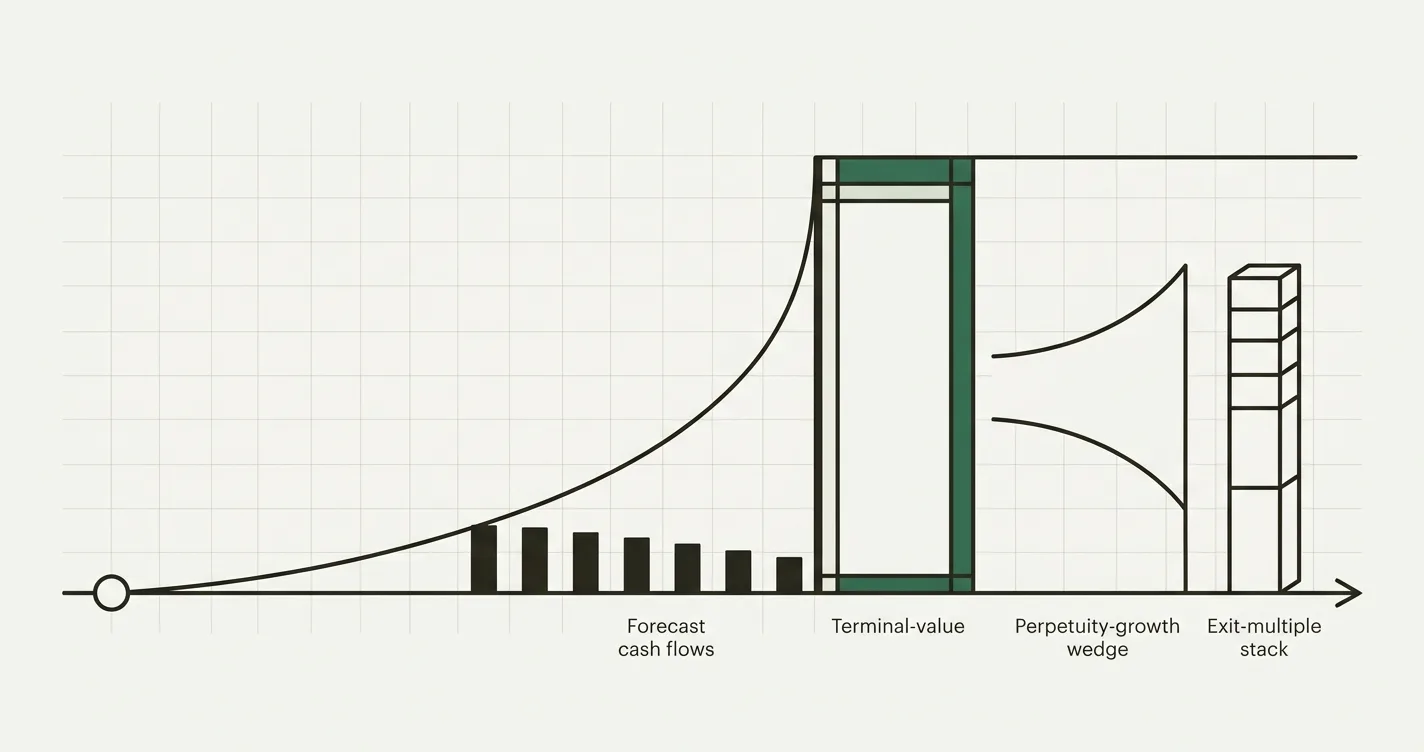
Choosing and cross-checking a terminal value method.
Why Terminal Value Dominates a DCF
The mechanics are simple: a DCF sums the present value of each forecast year's free cash flow, then adds the present value of the terminal value. The reason the terminal value usually wins is that it represents an infinite tail of cash flows, while the explicit forecast covers only a handful of years.
Consider a company whose Year 5 unlevered free cash flow is $100M, discounted at a 9% WACC. The five explicit forecast years might sum to roughly $350-400M of present value. The terminal value - even after discounting it back five years - can easily exceed $1 billion of present value. The tail dwarfs the body.
This is not a flaw in the method; it reflects economic reality. But it has a sharp practical consequence: the terminal value is where small assumption errors do the most damage. A 0.5% change in the perpetual growth rate, or a single turn on the exit multiple, can move the whole valuation by 15-30%. That is why the rest of this guide is about getting two numbers - the terminal growth rate and the exit multiple - defensible and consistent with each other.
Method 1: The Gordon Growth (Perpetuity Growth) Method
The Gordon Growth method assumes that after the explicit forecast, free cash flow grows at a single constant rate forever. It is the present value of a growing perpetuity, valued as of the end of the final forecast year:
Terminal Value = FCF_final x (1 + g) / (WACC - g)
Where:
- FCF_final is the unlevered free cash flow in the last explicit forecast year (Year 5 here).
- g is the perpetual (terminal) growth rate.
- WACC is the weighted average cost of capital - the discount rate.
Note that the numerator is the next year's cash flow: FCF_final x (1 + g). The formula values a perpetuity that begins growing the year after your forecast ends.
Choosing the terminal growth rate
The terminal growth rate is the most abused input in all of valuation. The rule is simple: g must not exceed the long-run nominal growth rate of the economy - roughly 2-3% in developed markets. No company can outgrow the economy forever; if it could, it would eventually become larger than the economy itself. A safe default is 2.0-2.5%.
Two hard constraints fall out of the formula:
- If g >= WACC, the denominator is zero or negative and the formula breaks (it implies infinite value). This is a signal your assumptions are inconsistent, not a real result.
- The gap (WACC - g) is the lever. As g approaches WACC, the terminal value explodes. That sensitivity is exactly why you stress-test it.
Worked example
Assume our final-year (Year 5) unlevered free cash flow is $100M, WACC is 9.0%, and we use a terminal growth rate of 2.5%:
Terminal Value = $100M x (1 + 0.025) / (0.09 - 0.025)
             = $102.5M / 0.065
             = $1,576.9M
The Excel formula, with Year 5 FCF in B10, WACC in B2, and g in B3:
// Gordon Growth terminal value (as of end of Year 5)
= B10 * (1 + B3) / (B2 - B3)
Method 2: The Exit Multiple Method
The exit multiple method takes a market-based view: instead of assuming the company runs forever, it assumes you sell it at the end of the forecast at a multiple that comparable companies (or recent transactions) trade at. The most common metric is EV/EBITDA:
Terminal Value = EBITDA_final x Exit Multiple
This terminal value is already an enterprise value as of the end of the final forecast year - it does not need a net-debt adjustment at the terminal step (that bridge happens once, at the end of the DCF). For more on that bridge, see our guide on enterprise value vs equity value.
Choosing the exit multiple
Ground the multiple in comparable companies trading today, not in a hoped-for future re-rating. If mature peers in the sector trade at 9-11x EV/EBITDA, your exit multiple should sit in that range - and arguably toward the lower end, because by the terminal year the company is mature and slower-growing than the high-multiple names. Building the peer set is its own discipline; see comparable company analysis for how to assemble and normalise it.
Worked example
Assume our Year 5 EBITDA is $180M and comparable mature businesses trade at an 11.0x EV/EBITDA multiple:
Terminal Value = $180M x 11.0 = $1,980M
The Excel formula, with Year 5 EBITDA in B12 and the multiple in B4:
// Exit multiple terminal value (as of end of Year 5)
= B12 * B4
Cross-Checking: Implied Multiple and Implied Growth
Here is the technique that separates an institutional DCF from a student one: run each method against the other. The two terminal values above ($1,576.9M from Gordon Growth, $1,980M from the exit multiple) disagree by 26%. Which one is right? Cross-checking tells you whether either is defensible.
Implied exit multiple (from a Gordon Growth TV)
Take the Gordon Growth terminal value and divide it by final-year EBITDA to see what exit multiple it implies:
Implied Exit Multiple = Terminal Value / EBITDA_final
                     = $1,576.9M / $180M
                     = 8.8x
So a 2.5% perpetual growth assumption implies an 8.8x exit multiple. If peers trade at 11x, the Gordon Growth result is conservative - which is usually a feature, not a bug.
Implied perpetuity growth (from an exit-multiple TV)
Now reverse it. Take the exit-multiple terminal value and back out the perpetual growth rate it implies. Rearranging the Gordon Growth formula to solve for g:
g = (Terminal Value x WACC - FCF_final) / (FCF_final + Terminal Value)
  = ($1,980M x 0.09 - $100M) / ($100M + $1,980M)
  = ($178.2M - $100M) / $2,080M
  = 3.8%
The 11x exit multiple implies a 3.8% perpetual growth rate - above the 2-3% economy ceiling. That is a red flag: it tells you the 11x multiple is slightly rich for a terminal-year business, and you should probably anchor toward the Gordon Growth answer or lower the multiple.
// Implied exit multiple from a Gordon Growth TV (TV in B14, EBITDA in B12)
= B14 / B12

// Implied perpetuity growth from an exit-multiple TV (TV in B16, WACC in B2, FCF in B10)
= (B16 * B2 - B10) / (B10 + B16)
When the implied multiple and implied growth both land in sensible ranges, you have a terminal value you can defend in front of an investment committee.
Discounting Terminal Value to Present Value
Both methods produce a value as of the end of the final forecast year (Year 5). To bring it into today's money, discount it by the same factor you apply to that year's cash flow:
PV of Terminal Value = Terminal Value / (1 + WACC) ^ N
With N = 5 years and WACC = 9.0%, the Year 5 discount factor is:
Discount Factor = 1 / (1.09) ^ 5 = 0.6499
Applying it to both terminal values:
| Method | Terminal Value (Year 5) | Discount Factor | PV of Terminal Value |
|---|---|---|---|
| Gordon Growth (g = 2.5%) | $1,576.9M | 0.6499 | $1,024.9M |
| Exit Multiple (11.0x) | $1,980.0M | 0.6499 | $1,286.9M |
// Present value of terminal value (TV in B14, WACC in B2, forecast years N in B5)
= B14 / (1 + B2) ^ B5
A note on mid-year convention. If you discount the explicit forecast cash flows using a mid-year convention (assuming cash arrives mid-period rather than at year-end), you must decide how to treat the terminal value. A common approach is to discount the terminal value by the full N periods (because it sits at the period boundary), while a stricter approach discounts it by N - 0.5 to stay consistent with the mid-year cash flows. Either is defensible - the cardinal rule is to pick one, apply it consistently, and document it. Don't silently mix conventions.
Worked Example: Both Methods Side by Side
Putting the full picture together for our example company - a five-year DCF where the explicit forecast cash flows discount to a present value of $380M:
| Component | Gordon Growth | Exit Multiple |
|---|---|---|
| PV of forecast UFCF (Years 1-5) | $380.0M | $380.0M |
| Terminal value (end of Year 5) | $1,576.9M | $1,980.0M |
| PV of terminal value | $1,024.9M | $1,286.9M |
| Enterprise Value | $1,404.9M | $1,666.9M |
| Terminal value as % of EV | 73% | 77% |
| Implied exit multiple | 8.8x | 11.0x |
| Implied perpetuity growth | 2.5% | 3.8% |
Notice the terminal value is 73-77% of enterprise value in both cases - textbook for a stable business, and a reminder of where the valuation risk really sits. The two methods bracket a range of roughly $1.40bn - $1.67bn of enterprise value, with a midpoint near $1.54bn. Present that range, not a single point.
To bridge from enterprise value to equity value, subtract net debt - the final step covered in detail in our DCF model tutorial. You can explore the full mechanics, including the terminal value block, in the live model below.
Sensitivity of Terminal Value
Because terminal value is so dominant, a sensitivity table on the two inputs that drive it - WACC and the terminal growth rate - is mandatory. The table below shows the undiscounted Gordon Growth terminal value (Year 5 value) for our $100M final-year cash flow across a grid of WACC and growth assumptions:
| WACC \ Terminal Growth | 1.5% | 2.0% | 2.5% | 3.0% | 3.5% |
|---|---|---|---|---|---|
| 8.0% | $1,562M | $1,700M | $1,864M | $2,060M | $2,300M |
| 8.5% | $1,450M | $1,569M | $1,708M | $1,873M | $2,070M |
| 9.0% | $1,353M | $1,457M | $1,577M | $1,717M | $1,882M |
| 9.5% | $1,269M | $1,360M | $1,464M | $1,585M | $1,725M |
| 10.0% | $1,194M | $1,275M | $1,367M | $1,471M | $1,592M |
The bold cell ($1,577M) is our base case (9.0% WACC, 2.5% growth). Read across the row and the terminal value rises 39% from the lowest to highest growth assumption; read down the column and it falls 24% as WACC rises. The grid spans $1.19bn to $2.30bn - nearly 2x - off changes that each look trivially small in isolation. That spread is the whole argument for stress-testing.
For the mechanics of building these tables natively in Excel, see our walkthrough of sensitivity analysis in Excel.
Common Mistakes to Avoid
- Terminal growth rate above the economy's growth. Using 4-5% perpetual growth in a developed market implies the company eventually swallows the entire economy. Cap g at long-run nominal GDP growth (2-3%).
- g greater than or equal to WACC. This breaks the formula and produces negative or infinite values. If you see it, your assumptions are inconsistent - it is not a real number.
- Never cross-checking the two methods. A Gordon Growth TV that implies a 20x exit multiple, or an exit multiple that implies 5% perpetual growth, is telling you something is wrong. Always back out the implied figure.
- Using a non-normalised final-year cash flow. If Year 5 has unusually high CapEx, a working-capital swing, or a one-off, the perpetuity inherits that distortion forever. Normalise the final-year cash flow (steady-state CapEx roughly equal to depreciation, normalised margins) before applying the perpetuity.
- Forgetting to grow the numerator. The Gordon Growth formula uses FCF x (1 + g), not bare FCF. Dropping the (1 + g) understates the terminal value.
- Discounting the terminal value to the wrong period. The TV sits at the end of Year N, so it is discounted by N periods - not N + 1. And keep the mid-year convention consistent between the explicit cash flows and the terminal value.
- Presenting a single point. Given the sensitivity, a single terminal value (and therefore a single valuation) is false precision. Show a range from both methods and a sensitivity table.
- Stale exit multiples. Anchoring the exit multiple to today's high-growth peers rather than mature, terminal-year-appropriate comparables systematically overstates value.

Alex Tapio
Founder of Finamodel • Professional Financial Modeller • Ex-Deloitte