Budget vs Actual (Variance) Analysis: How to Build One in Excel
Key Takeaways
- Variance is Actual minus Budget - but the meaning flips. A positive dollar variance is favorable for revenue and unfavorable for costs. Encode a P&L-impact column so favorable is always positive and one flag works across the statement.
- Favorable is not the same as good. A green cost cell can be skipped investment; a green revenue cell can be a margin-killing discount. Always read a variance next to its driver.
- Decompose material revenue variances into price and volume. (Actual Units − Budget Units) × Budget Price and (Actual Price − Budget Price) × Actual Units sum to the total, and they tell opposite stories about the same beat.
- Use a flexible budget when volume moves. Re-stating the budget at actual volume splits the static-budget variance into an expected sales-volume piece and the true, controllable spending variance - the only one worth managing.
- Investigate by exception, on two thresholds. Require a variance to breach both a dollar amount and a percentage before it earns a root-cause review. That keeps the analysis on the handful of gaps that move the P&L.
- Close the loop. The output of variance analysis is a corrected assumption. Feed material, recurring variances back into the forecast so the next cycle is more accurate - that feedback is what turns a report into a management tool.
Budget vs actual analysis is the discipline of comparing what you planned - your budget - against what actually happened, then explaining every meaningful gap. That gap is the variance, and turning it into insight is the core feedback loop of FP&A. This guide shows you how to build a budget vs actuals report in Excel: calculate favorable and unfavorable variances, decompose a revenue miss into price and volume, separate a static-budget variance from a true spending variance with a flexible budget, and decide which variances are actually worth investigating.
A budget is a promise the business makes once a year; actuals are what it delivers month after month. Budget vs actual analysis - often just called variance analysis - is how you hold the two up against each other and ask the only question that matters in FP&A: where did reality diverge from plan, and why?
Done well, it is a management tool, not an accounting chore. A clean variance report tells a CFO exactly which lines beat plan, which missed, whether a miss was driven by price or by volume, and which gaps are large enough to act on. Done badly, it is a wall of red and green with no story - every line flagged, nothing prioritised, no root cause. The difference is structure, and that is what this guide builds.
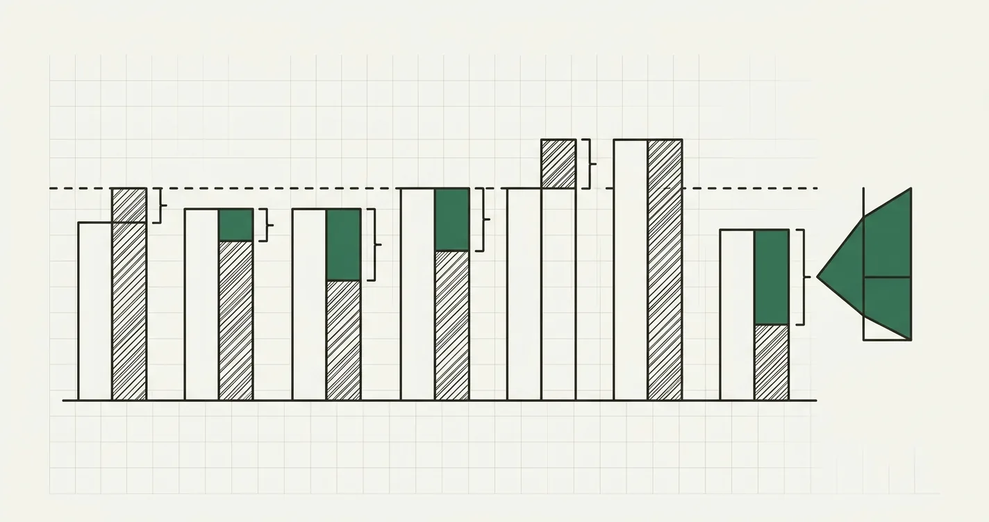
The budget vs actuals workflow: measure the gap, filter for materiality, decompose the drivers, act, and re-forecast.
The Core Variance Formula
Every variance starts from one subtraction:
Dollar Variance = Actual - Budget
Percentage Variance = (Actual - Budget) / Budget
The arithmetic is trivial; the interpretation is where people slip. A positive dollar variance means different things depending on the line item. If actual revenue comes in above budget, that is good. If an actual cost comes in above budget, that is bad - even though both are 'positive' in raw dollars. This is the favorable / unfavorable distinction, and it flips between the top and bottom of the P&L:
| Line type | Actual > Budget | Actual < Budget |
|---|---|---|
| Revenue / profit | Favorable | Unfavorable |
| Cost / expense | Unfavorable | Favorable |
A favorable variance improves profit relative to plan; an unfavorable variance reduces it. The safest way to encode this in a model is a single P&L-impact column that always makes favorable positive - subtract in the direction that matters for each line type - so one flag works across the whole statement. We will build exactly that below.
A Worked Budget vs Actuals Report
Here is a one-month operating statement for a mid-sized business. Budget was set at the start of the year; actuals just closed. The report computes the dollar variance, the percentage variance, and a favorable/unfavorable flag for each line.
| Line item | Budget | Actual | Variance ($) | Variance (%) | F / U |
|---|---|---|---|---|---|
| Revenue | $500,000 | $520,000 | +$20,000 | +4.0% | Favorable |
| COGS | $200,000 | $215,000 | +$15,000 | +7.5% | Unfavorable |
| Gross Profit | $300,000 | $305,000 | +$5,000 | +1.7% | Favorable |
| Operating Expenses | $180,000 | $172,000 | −$8,000 | −4.4% | Favorable |
| Operating Income | $120,000 | $133,000 | +$13,000 | +10.8% | Favorable |
Read it as a story rather than a grid. Revenue beat plan by $20,000 (+4.0%) - favorable. But COGS ran $15,000 over budget (+7.5%) - unfavorable, and it ate into the revenue beat, leaving gross profit only $5,000 (+1.7%) ahead. The rescue came below the gross-profit line: operating expenses came in $8,000 under budget (−4.4%, favorable), which lifted operating income to $133,000 - $13,000 (+10.8%) above plan. The headline is good, but the mix is worth a second look: the profit beat was carried by an opex underspend, while the core product economics (COGS as a share of revenue) actually deteriorated.
The Excel formulas
Lay the report out with budget in column B and actual in column C. Add a hidden Type column (A) tagging each row 'Revenue' or 'Cost' so the favorable/unfavorable logic is data-driven rather than hand-typed:
// Dollar variance
= C2 - B2

// Percentage variance, guarded against a zero budget
= IF(B2 = 0, "n/a", (C2 - B2) / B2)

// P&L impact: favorable is always positive
// Revenue lines: Actual − Budget; Cost lines: Budget − Actual
= IF(A2 = "Revenue", C2 - B2, B2 - C2)

// Favorable / Unfavorable label, read off the impact column (D)
= IF(D2 >= 0, "Favorable", "Unfavorable")
Because the flag reads from the P&L-impact column, it stays correct whether the row is revenue or cost - no manual overrides, no accidental green on a cost overrun.
Favorable Isn't Always Good
The favorable/unfavorable flag answers did this line help or hurt profit versus plan - not is this a good outcome. Two traps hide behind a green cell:
- A favorable cost variance can be underinvestment. Marketing came in $30,000 under budget because the team never launched the campaign; R&D is favorable because a key hire slipped a quarter. The variance is favorable this month and expensive later.
- A favorable revenue variance can be a margin problem. Beating the revenue budget by discounting hard to push volume looks favorable on the top line while quietly compressing gross margin.
That second trap is exactly why a top-line variance is not enough. You have to open it up and ask whether the beat came from selling more or from charging differently. That is variance decomposition.
Decomposing the Variance: Price vs Volume
A revenue variance has two independent causes: you sold a different quantity than planned (volume), and you sold at a different price (price). Decomposing the total into those two pieces turns a single number into a diagnosis.
The standard two-way split values the volume effect at the budgeted price and the price effect at the actual volume:
Volume Variance = (Actual Units - Budget Units) × Budget Price
Price Variance  = (Actual Price - Budget Price) × Actual Units
The two always sum back to the total revenue variance. Take a product line budgeted at 10,000 units at $50.00, where actuals landed at 11,000 units at $48.00:
| Units | Price | Revenue | |
|---|---|---|---|
| Budget | 10,000 | $50.00 | $500,000 |
| Actual | 11,000 | $48.00 | $528,000 |
| Total variance | +$28,000 |
On the surface, a $28,000 favorable revenue variance - a clean beat. Now decompose it:
| Component | Formula | Calculation | Variance | F / U |
|---|---|---|---|---|
| Volume variance | (Actual Units − Budget Units) × Budget Price | (11,000 − 10,000) × $50.00 | +$50,000 | Favorable |
| Price variance | (Actual Price − Budget Price) × Actual Units | ($48.00 − $50.00) × 11,000 | −$22,000 | Unfavorable |
| Total revenue variance | +$28,000 | Favorable |
The decomposition rewrites the story completely. The business did not simply beat plan by $28,000 - it sold +$50,000 of extra volume while giving back −$22,000 on price. The headline beat is real, but it was bought with a discount: the team moved 10% more units by cutting price 4%. Whether that is a win depends on the margin on those extra units - a question the top-line number alone could never raise.
// Volume variance: the extra units valued at the budgeted price
= (Actual_Units - Budget_Units) * Budget_Price

// Price variance: the price change valued at the actual units
= (Actual_Price - Budget_Price) * Actual_Units
The same idea applies to costs, where the split is usually called rate and efficiency: a rate variance (paid a different price per hour or per unit of input) and an efficiency variance (used more or fewer inputs than the standard). The mechanics are identical - hold one factor at standard, flex the other.
Static vs Flexible Budget Variance
There is a deeper problem with comparing actuals straight to the original budget: the budget was built for one activity level, and actual activity is almost never exactly that. When volume differs, a raw comparison blends two things you want to keep apart - how much you did and how well you did it. The fix is a flexible budget: re-state the budget at the actual volume, using the original per-unit rates.
Suppose variable production cost was budgeted at $30.00 per unit. The static budget assumed 10,000 units; actual output was 11,000 units at a total actual cost of $345,000.
| Volume | Variable cost | |
|---|---|---|
| Static budget | 10,000 units | $300,000 |
| Flexible budget (actual volume × budgeted rate) | 11,000 units | $330,000 |
| Actual | 11,000 units | $345,000 |
Now split the total gap into its two meaningful pieces:
| Variance | Formula | Calculation | Result |
|---|---|---|---|
| Static-budget variance | Actual − Static budget | $345,000 − $300,000 | $45,000 U |
| Sales-volume variance | Flexible budget − Static budget | $330,000 − $300,000 | $30,000 |
| Flexible-budget variance | Actual − Flexible budget | $345,000 − $330,000 | $15,000 U |
The naïve read of the static-budget variance is alarming: costs overran by $45,000. But $30,000 of that is simply the expected cost of producing 10% more units - and if you made more because you sold more, revenue rose to match. Only the $15,000 flexible-budget variance is a genuine, controllable overspend. On a per-unit basis it is $345,000 / 11,000 = $31.36 actual against a $30.00 standard - a $1.36 per-unit overrun across 11,000 units. That $15,000 is the number a plant manager should be held to; the $45,000 headline would have sent the review chasing a problem that is two-thirds phantom.
// Flexible budget = actual volume × budgeted cost per unit
= Actual_Units * Budget_Cost_Per_Unit

// Flexible-budget (spending / efficiency) variance
= Actual_Cost - Flexible_Budget

// Sales-volume variance (the piece caused purely by activity level)
= Flexible_Budget - Static_Budget
Which Variances to Investigate
A month-end statement can throw off dozens of variances. Chasing all of them wastes the team and buries the two or three that matter. The discipline is management by exception: set a materiality threshold and only investigate variances that breach it.
Use two thresholds together - an absolute dollar amount and a percentage - and require both. Requiring both filters out the two kinds of noise: large-dollar but small-percent gaps on big line items that are actually within tolerance, and large-percent but small-dollar gaps on trivial line items. Applying a '$10,000 and 5%' rule to the operating statement above:
| Line | Variance ($) | Variance (%) | > $10,000? | > 5%? | Action |
|---|---|---|---|---|---|
| Revenue | +$20,000 | 4.0% | Yes | No | Monitor |
| COGS | +$15,000 | 7.5% | Yes | Yes | Investigate |
| Operating Expenses | −$8,000 | 4.4% | No | No | Monitor |
Only COGS trips both wires, and it is exactly the line the earlier read flagged as the real weakness. The revenue beat is big in dollars but a modest 4% - within tolerance. The opex saving is a small $8,000. The 'and' logic sends the analyst straight to the one variance worth a root-cause investigation.
// Management-by-exception flag: material on BOTH dollars and percent
= IF(
    AND( ABS(C2 - B2) > 10000, ABS((C2 - B2) / B2) > 0.05 ),
    "Investigate",
    "Monitor"
  )
Building the Report in Excel
A variance report is only useful if a busy reader can scan it in seconds. A few formatting habits do most of the work:
- Colour by exception, not by cell. Do not paint every variance red or green - that just creates visual noise. Use conditional formatting to highlight only the rows flagged 'Investigate', so the eye lands on the exceptions.
- Show both dollars and percent, side by side. A dollar figure without a percentage hides scale; a percentage without dollars hides significance. The pair together is what makes the materiality judgement obvious.
- Keep the F/U flag formula-driven. Never hand-type 'Favorable' - derive it from the P&L-impact column so it can never contradict the numbers.
- Add a short commentary column. The most valuable cell in the report is the one-line explanation next to each material variance. Numbers show what moved; the commentary is where FP&A earns its keep by saying why.
The budget-vs-actuals template below wires all of this together - budget and actual inputs, automatic dollar and percentage variances, a favorable/unfavorable flag, and an exception highlight - so you can drop in your own numbers rather than rebuild the scaffolding.
Closing the Loop: From Variance to Re-Forecast
A variance report that ends at 'here is the gap' throws away most of its value. The point of measuring the variance is to change the next number. Each month the loop should run: measure the variance, decompose the material ones, identify the root cause, then decide whether the gap is a one-off (a timing shift, a one-time cost) or a signal that a forecast assumption is wrong.
When it is a signal, feed it back. If COGS is running 7.5% over plan because input prices rose, the forward forecast - and the budget assumptions inside your operating model - should reflect the new cost per unit, not the stale one. That is the difference between a static annual budget that decays into irrelevance by Q3 and a rolling forecast that stays current. Variance analysis is the mechanism that keeps the full 3-statement financial model honest, because it is the check that tells you which of its assumptions reality has already overturned.
For the forecasting side of the same loop - how to build the projections you are measuring against - see our guide to financial forecasting methods, which walks through driver-based forecasting and how to score forecast accuracy with MAPE once the actuals land.
Common Mistakes to Avoid
- Reading the top line and stopping. A favorable revenue variance can hide an unfavorable price variance underneath. Always decompose a material revenue gap into price and volume before you call it a win.
- Comparing actuals to a static budget when volume moved. If actual activity differs from plan, the raw variance conflates volume and efficiency. Flex the budget to actual volume so the spending variance you manage is the controllable one.
- Confusing 'favorable' with 'good'. A cost underspend can be underinvestment; a revenue beat can be a discount. The flag measures P&L impact versus plan, not business health - read it with its cause.
- Flagging everything. Painting every cell red or green and investigating every gap buries the two variances that matter. Use a dual dollar-and-percent materiality threshold and management by exception.
- Using a single threshold. A percentage-only rule chases trivial dollar swings on small lines; a dollar-only rule misses large-percent problems on small lines. Require both to breach before you investigate.
- Hardcoding the favorable/unfavorable flag. Typing 'Favorable' by hand guarantees that sooner or later it contradicts the numbers. Derive every label from a P&L-impact formula.
- Never closing the loop. A variance you explain but never feed back into the forecast is a lesson wasted. The output of this month's analysis should be next month's better assumption.

Alex Tapio
Founder of Finamodel • Professional Financial Modeller • Ex-Deloitte