Financial Forecasting Methods Explained: How to Build a Financial Forecast
Key Takeaways
- A forecast is an estimate built from assumptions, not an extrapolation of the past. The method you choose decides whether it can withstand scrutiny.
- Time-series methods (straight-line, moving average, linear trend) are fast sanity checks. They work when history is clean and the trend is stable, and they converge - when they disagree, the trend is breaking.
- Driver-based forecasting is the FP&A standard. Decomposing revenue into units × price (and costs into their own drivers) makes every assumption explicit, enables real scenario analysis, and reveals dynamics like operating leverage that flat-growth forecasts hide.
- Build bottom-up, reconcile top-down. Your own operational data is the more defensible foundation; the market view is the reality check on whether your implied share is sane.
- Centralise assumptions, never hardcode. A change to one input should ripple through the whole model instantly. That is what makes a forecast auditable and scenario-ready.
- Close the loop with budget-vs-actuals. Measure forecast accuracy with MAPE, watch for bias, and feed every variance back into the next cycle - that feedback is how forecasting becomes a skill rather than a guess.
- Roll the forecast forward. A static annual budget decays; a rolling forecast keeps a constant horizon and stays continuously current.
For the operational side of forecasting, see our guide to building a cash flow forecast in Excel, and for the foundations that any forecast plugs into, read how to build a 3-statement financial model. To stress-test your assumptions once the forecast is built, our sensitivity analysis in Excel walkthrough shows how to turn a single estimate into a defensible range.
A financial forecast is a forward-looking estimate of how a business will perform - its revenue, costs, profit, and cash - built from historical data and explicit assumptions. The method you choose determines how credible that forecast is. This guide walks through the four main financial forecasting methods, from quick straight-line extrapolation to the driver-based approach that FP&A teams rely on, with a full worked revenue forecast in Excel, the formulas to build it, and how to measure forecast accuracy once the actuals arrive.
Every budget, valuation, fundraising deck, and board pack rests on a financial forecast. Yet most forecasts fail for the same reason: they are extrapolations dressed up as analysis. Someone grows last year's revenue by a round number, copies the formula across, and calls it a plan. When reality diverges - as it always does - there is no way to know which assumption broke, because the forecast was never built from assumptions in the first place.
Good financial forecasting is different. It makes the logic explicit, ties the financial outcome to operational drivers management actually controls, and can be tested against actuals to get better over time. Choosing the right forecasting method for the situation is the first decision, and it matters more than the spreadsheet skills that follow.
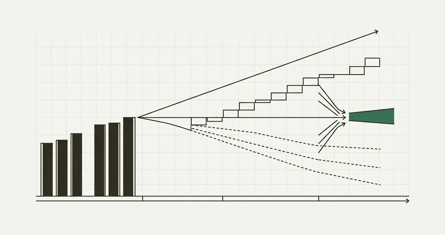
Choosing a financial forecasting method: the amount and quality of history, plus the stability of the trend, point you to the right approach.
Forecast vs. Budget vs. Projection
These three words get used interchangeably, but in FP&A they mean different things:
- Budget: A fixed financial target, set once (usually annually) and held constant. It is what you committed to.
- Forecast: Your best current estimate of what will actually happen, refreshed as new data arrives. It is what you now expect.
- Projection: A scenario-based 'what-if' that models a specific set of assumptions, often over a longer horizon (e.g., a 5-year projection for a valuation).
The budget is the yardstick; the forecast is the moving estimate you measure against it. The gap between them - the variance - is the single most useful number FP&A produces, because it tells you where the business is drifting from plan.
The Four Main Forecasting Methods
Financial forecasting methods sit on a spectrum from purely mechanical (extrapolate the past) to fully causal (build from drivers). Here is how they compare:
| Method | How it works | Best for | Weakness |
|---|---|---|---|
| Straight-line | Apply one growth rate (often the CAGR) to the last actual | Stable, mature lines; quick first-pass | Ignores changing dynamics; mechanical |
| Moving average | Average recent periods to smooth noise | Seasonal or noisy data; short horizons | Lags turning points; backward-looking |
| Linear trend / regression | Fit a statistical line through history | Series with a clear linear trend | Assumes the past pattern continues |
| Driver-based | Build line items from operational drivers | Anything you can decompose; scenario work | More work to build and maintain |
The first three are time-series methods - they look only at the history of the number itself. The fourth, driver-based forecasting, looks at why the number moves. For any forecast that has to survive scrutiny - a board, an investor, a lender - driver-based is the standard. The time-series methods are best used as fast sanity checks against it.
Methods 1–3: Forecasting from History
When you have several clean periods of history and the trend is reasonably stable, time-series methods give you a quick estimate. Take this five-year revenue history:
| Year | Revenue ($M) | YoY Growth |
|---|---|---|
| Year 1 | $100.0M | - |
| Year 2 | $118.0M | +18.0% |
| Year 3 | $131.0M | +11.0% |
| Year 4 | $152.0M | +16.0% |
| Year 5 | $168.0M | +10.5% |
Let's forecast Year 6 three different ways.
Straight-Line (CAGR)
The straight-line method applies a single compound growth rate to the last actual. The most defensible rate is the historical CAGR:
CAGR = (End Value / Start Value) ^ (1 / Periods) - 1
CAGR = (168 / 100) ^ (1 / 4) - 1 = 13.8%

Year 6 Forecast = $168.0M × (1 + 0.138) = $191.3M
// CAGR from a history range (revenue in B2:B6, 4 periods of growth)
= (B6 / B2) ^ (1 / 4) - 1

// Year 6 straight-line forecast
= B6 * (1 + $B$8)   // B8 holds the CAGR
Moving Average (of Growth)
A moving average smooths recent periods. Here we average the last three YoY growth rates (11.0%, 16.0%, 10.5% = 12.5%) and apply it:
Year 6 Forecast = $168.0M × (1 + 0.125) = $189.0M
// 3-year average of the most recent growth rates (in C4:C6)
= AVERAGE(C4:C6)

// Apply it to the last actual
= B6 * (1 + AVERAGE(C4:C6))
Linear Trend (Regression)
The linear-trend method fits a regression line through the history and extends it. Excel does this natively with FORECAST.LINEAR (or TREND):
// Periods 1-5 in A2:A6, revenue in B2:B6; forecast period 6
= FORECAST.LINEAR(6, B2:B6, A2:A6)

// TREND does the same and can output multiple future periods at once
= TREND(B2:B6, A2:A6, 6)
For this series the regression slope is $17.0M per year with an intercept of $82.8M, so:
Year 6 Forecast = $82.8M + $17.0M × 6 = $184.8M
Comparing the Three
| Method | Year 6 Forecast | When to trust it |
|---|---|---|
| Straight-line (CAGR 13.8%) | $191.3M | Stable compounding growth |
| Moving average (12.5%) | $189.0M | Recent periods most representative |
| Linear trend (regression) | $184.8M | Steady absolute (not %) growth |
The three answers land within ~3.5% of each other - which is the tell that this series is stable and any of them is defensible. When time-series methods disagree sharply, that is your signal the trend is breaking and a mechanical extrapolation will mislead you. That is exactly when you reach for driver-based forecasting.
Method 4: Driver-Based Forecasting (The FP&A Standard)
Driver-based forecasting abandons extrapolation of the output and instead forecasts the inputs that produce it. Revenue is not a number that grows 13% a year - it is units sold multiplied by average selling price, each of which has its own logic. Decomposing the forecast this way makes every assumption visible, debatable, and scenario-ready.
Worked Example: A Driver-Based Revenue and Margin Forecast
Let's build a five-year forecast for a consumer-products company from the ground up. Every input lives on an Assumptions sheet:
| Driver | Value |
|---|---|
| Year 1 units sold | 1,000,000 |
| Unit growth (Y2–Y5) | 12%, 10%, 9%, 8% |
| Year 1 average selling price (ASP) | $50.00 |
| ASP growth | 3% per year |
| Gross margin | 42% of revenue |
| Variable opex | 10% of revenue |
| Fixed opex (Year 1) | $8.0M, growing 4% per year |
Revenue is the product of two independent drivers - units and price:
Revenue = Units Sold × Average Selling Price
Working the drivers forward gives a full mini-P&L:
| Metric | Year 1 | Year 2 | Year 3 | Year 4 | Year 5 |
|---|---|---|---|---|---|
| Units Sold | 1.000M | 1.120M | 1.232M | 1.343M | 1.450M |
| ASP | $50.00 | $51.50 | $53.05 | $54.64 | $56.28 |
| Revenue | $50.0M | $57.7M | $65.4M | $73.4M | $81.6M |
| Gross Profit (42%) | $21.0M | $24.2M | $27.5M | $30.8M | $34.3M |
| Variable Opex (10% Rev) | $5.0M | $5.8M | $6.5M | $7.3M | $8.2M |
| Fixed Opex (+4%/yr) | $8.0M | $8.3M | $8.7M | $9.0M | $9.4M |
| Operating Income | $8.0M | $10.1M | $12.3M | $14.5M | $16.8M |
| Operating Margin | 16.0% | 17.6% | 18.7% | 19.7% | 20.5% |
Notice what the driver-based structure reveals that a straight-line forecast hides: operating margin expands from 16.0% to 20.5% - not because we assumed it, but because fixed costs grow slower than revenue (operating leverage). A flat growth-rate forecast on operating income would have missed that entirely.
The Excel Formulas
Each driver compounds off the prior period, and outputs reference the Assumptions sheet - never a hardcoded number:
// Units: prior year × (1 + unit growth assumption)
= D_Units_PriorYear * (1 + Assumptions!$C$3)

// ASP: prior year × (1 + ASP growth)
= D_ASP_PriorYear * (1 + Assumptions!$C$5)

// Revenue: the two drivers multiplied
= Units * ASP

// Gross profit
= Revenue * Assumptions!$C$6

// Variable opex scales with revenue; fixed opex compounds on its own
= Revenue * Assumptions!$C$7
= FixedOpex_PriorYear * (1 + Assumptions!$C$8)

// Operating income
= GrossProfit - VariableOpex - FixedOpex
Because every output traces to an assumption cell, you can change one input - say, drop unit growth from 12% to 8% - and watch the entire five-year P&L and margin profile update instantly. That is the property time-series methods can never give you.
Top-Down vs. Bottom-Up Revenue Forecasting
The driver-based example above is a bottom-up revenue forecast: it builds from your own units and price. The alternative is top-down, which starts from the market:
Top-Down Revenue = Total Addressable Market (TAM) × Target Market Share
| Approach | Starts from | Best for | Risk |
|---|---|---|---|
| Bottom-up | Your units, customers, reps, traffic | Established operations with internal data | Can miss market ceiling |
| Top-down | TAM and market-share assumption | New markets, early-stage, new products | Share assumptions are easy to inflate |
The professional habit is to build bottom-up and then reconcile against top-down. If your bottom-up forecast implies you'll capture 40% of a market where the leader has 25%, the assumptions are wrong somewhere. For early-stage companies with no operating history, start top-down for the envelope, then switch to driver-based bottom-up as soon as you have real funnel data. Our startup financial model guide walks through that transition in detail.
Closing the Loop: Budget vs. Actuals and Forecast Accuracy
A forecast you never check is just a guess. The discipline that turns forecasting into a skill is the budget-vs-actuals review: every month, compare what you forecast to what happened, isolate the variance, and feed the lesson back into next month's numbers.
Measuring Forecast Accuracy
The standard accuracy metric is MAPE (Mean Absolute Percentage Error) - the average absolute miss as a percentage of actuals:
MAPE = AVERAGE( | Actual - Forecast | / Actual )
Forecast Accuracy = 100% - MAPE
Here is a three-month example:
| Month | Forecast | Actual | Variance | Abs % Error |
|---|---|---|---|---|
| January | $100.0k | $96.0k | −$4.0k | 4.2% |
| February | $105.0k | $110.0k | +$5.0k | 4.5% |
| March | $110.0k | $103.0k | −$7.0k | 6.8% |
| MAPE | - | - | - | 5.2% |
A 5.2% MAPE means forecast accuracy of 94.8% - strong for monthly revenue.
// Absolute percentage error per row (forecast in B, actual in C)
= ABS(C2 - B2) / C2

// MAPE across the range
= AVERAGE(D2:D4)
Also track bias - the average signed error. A low MAPE with persistently positive variances means you are systematically over-forecasting, which a pure accuracy number hides. In the example above the signed variances are −4, +5, −7 (net negative), so this forecaster runs slightly conservative.
Static Budget vs. Rolling Forecast
Most companies still set an annual budget and hold it for twelve months - by Q4 it bears little resemblance to reality. A rolling forecast fixes this: every month (or quarter) you drop the oldest period and add a new one, always keeping a constant 12- or 18-month horizon. It costs more effort but keeps the forecast continuously current, which is why driver-based models - fast to re-run - pair naturally with rolling forecasts.
Common Mistakes to Avoid
- Extrapolating instead of forecasting. Growing every line by a flat rate is fast and almost always wrong. If you can't say why a number grows, you don't have a forecast - you have a trend line.
- Hardcoding assumptions into formulas. The instant you type a growth rate directly inside a revenue formula, the model becomes un-auditable and scenarios become impossible. Every driver belongs on the
Assumptionssheet. - One method, no sanity check. A single driver-based forecast is far stronger when you cross-check it against a quick straight-line or top-down estimate. Big divergences flag bad assumptions early.
- Confusing the budget with the forecast. Holding a stale annual budget as your 'forecast' for ten months means you are flying on out-of-date information. Refresh the forecast; keep the budget as the yardstick.
- Ignoring variance. A forecast that is never compared to actuals never improves. Skipping the budget-vs-actuals review throws away the only feedback loop you have.
- Equal precision across the horizon. Treating month 36 of a forecast as reliably as month 1. Detail the near term; simplify the long term - and say so.
- Optimism creep. Forecasts drift high because every assumption gets the benefit of the doubt. Track bias, not just accuracy, and the pattern shows up fast.

Alex Tapio
Founder of Finamodel • Professional Financial Modeller • Ex-Deloitte