How to Build a Debt Schedule in Excel
Key Takeaways
- One identity runs the whole model: Closing = Opening + Draws − Scheduled Principal − Cash Sweep + PIK Accrual, applied per tranche, per period.
- One type code, three profiles: a single code (bullet, linear, sweep) drives the scheduled-principal formula, so any instrument drops in by setting face, maturity, and type - no rewiring.
- Break the revolver circularity deliberately: compute interest on the opening balance to avoid the loop, or knowingly enable iterative calculation. Never leave it broken.
- PIK is quiet until it isn't: PIK interest compounds onto the balance and only repays at maturity. A $20M note at 10% PIK becomes $32.2M in five years - model the accrual explicitly.
- Covenants are half the model: compute leverage, interest coverage, and DSCR every period with pass / watch / breach flags. The tightest year is usually early, when amortization and sweeps stack up.
- Feed the three statements from one source: closing debt to the balance sheet, total interest to the income statement, and draws, principal, and sweep to financing cash flows - all from the same roll-forward, so they can never disagree.
To see the debt schedule working inside a complete leveraged model, read our LBO model tutorial, and for the statement linkages it feeds, our guide to the 3-statement financial model. You can also download the full debt schedule template to build on.
A debt schedule is the engine room of any leveraged financial model. It takes a stack of debt tranches - a revolver, term loans, senior notes, a mezzanine PIK piece - and rolls each one forward period by period: opening balance, new draws, scheduled principal, cash sweep, PIK accrual, closing balance. From that roll-forward flow the interest expense on your income statement, the debt line on your balance sheet, and the financing cash flows on your cash flow statement. This guide walks through the full mechanic in Excel, the three amortization profiles, revolver and cash-sweep modeling, PIK interest, a fully worked two-tranche example, and the leverage, coverage, and DSCR covenant tests that lenders actually monitor.
Every model with leverage lives or dies on its debt schedule. In an LBO, the debt schedule is where sponsor returns are won or lost - how fast the business deleverages drives the equity multiple. In a 3-statement model, the debt schedule is what keeps the balance sheet balancing as the company borrows and repays. And in credit analysis, the debt schedule is where covenants are tested quarter by quarter to confirm the borrower stays inside its agreement.
The reason a debt schedule deserves its own sheet - rather than a few formulas buried in the balance sheet - is that a single debt tranche touches all three statements. Get it wrong in one place and the whole model breaks. Build it once, cleanly, and it becomes the single source of truth for everything debt-related.
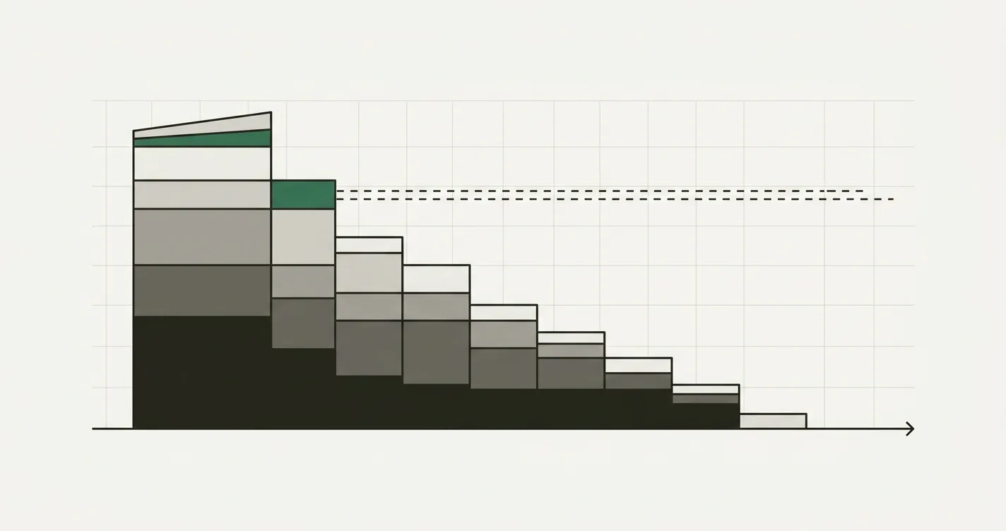
The Debt Schedule Roll-Forward: how each period chains from opening to closing balance and feeds the three statements
What a Debt Schedule Actually Does
A debt schedule answers one question for every debt instrument, in every period: how much is outstanding, how much interest accrued, and how much principal moved? Formally, it is a roll-forward:
Closing Balance = Opening Balance + Draws - Scheduled Principal - Cash Sweep + PIK Accrual
That one identity, applied tranche by tranche and period by period, is the entire model. Everything else - the interest schedule, the covenant tests, the dashboard - is derived from it. The professional versions run monthly over 60 months and stack five or more tranches; the logic is identical to the annual, two-tranche version we will build below.
Structuring the Schedule in Excel
A clean debt schedule follows a consistent sheet architecture:
- Assumptions / Input panel: One row per tranche holding face amount, draw month, maturity month, cash interest rate, PIK rate, amortization type code, initial draw percent, cash sweep rate, and commitment fee. Plus the operating inputs the covenants need: an EBITDA path and a cash-flow conversion factor.
- Debt Schedule: One block of rows per tranche (opening, draw, scheduled principal, sweep, PIK, closing) across the forecast horizon, with a panel-total block at the bottom summing all tranches.
- Interest Schedule: Per-tranche cash interest, PIK interest, and commitment fee, again with a panel total.
- Covenants: Trailing-twelve-month leverage, interest coverage, and DSCR with pass / watch / breach status flags.
- Dashboard: Peak debt, blended rate, total interest paid, average DSCR, peak leverage, weighted-average maturity, and breach counts.
The golden rule is the same as any financial model: never hardcode a number inside a formula. Every rate, face amount, and maturity lives on the input panel, and every schedule formula references it. This is what lets you re-size a debt stack in seconds and stress-test refinancing risk without rewiring anything. For the broader discipline, see our guide to Excel financial modeling best practices.
The Roll-Forward Mechanic, Formula by Formula
Each tranche gets six rows. Here is how each one is built in Excel, assuming your periods run across columns.
Opening balance is simply the prior period's closing balance:
// Opening = prior period closing (same tranche)
= C15
Scheduled principal resolves by the tranche's type code. A single nested formula handles all three profiles (1 = bullet, 2 = linear, 3 = sweep):
= IF(Type=1, IF(Month=Maturity, Opening, 0),
   IF(Type=2, IF(AND(Month>Draw_Month, Month<=Maturity), Face/(Maturity-Draw_Month), 0),
   0))
Bullet tranches repay everything at maturity; linear tranches repay an equal slice each period; sweep tranches return zero here because their principal is handled separately.
Cash sweep applies only to sweep-type tranches (the revolver). It uses excess cash flow, capped at the opening balance so the balance can never go negative:
// Excess cash = CFADS - cash interest - mandatory scheduled principal
= MIN(Excess_Cash * Sweep_Rate, Opening_Balance)
PIK accrual compounds onto the balance for tranches with a PIK rate:
= Opening_Balance * PIK_Rate
Closing balance ties the block together:
= Opening + Draw - Scheduled_Principal - Cash_Sweep + PIK_Accrual
And on the interest schedule, cash interest accrues on the opening balance:
= Opening_Balance * Cash_Rate
Using the opening balance for interest - rather than the average of opening and closing - is a deliberate choice. It keeps the interest calculation independent of the same period's sweep, which eliminates the circular reference that otherwise plagues debt schedules. More on that below.
The Three Amortization Profiles
Almost every real debt instrument fits one of three repayment profiles, and one type code drives all of them:
| Type | Code | Scheduled principal | Typical instrument |
|---|---|---|---|
| Bullet | 1 | Nothing until maturity, then the full balance | Senior notes, Term Loan B, high-yield bonds |
| Linear | 2 | Equal slice each period = Face / (Maturity − Draw) | Term Loan A, bank amortizing loans |
| Sweep | 3 | No scheduled amount; paid with excess cash | Revolving credit facility |
Because the type code drives the formula, you can drop any new instrument into the model by setting three cells - face, maturity, and type - without touching the schedule logic. That is what makes the model reusable across an LBO, a refinancing, and a 3-statement debt block.
Modeling the Revolver and the Cash Sweep
Revolver modeling is where most debt schedules break, because the revolver introduces a circular dependency. The revolver is drawn when the business is short of cash and swept down when it has excess cash. But the amount of excess cash depends on interest expense, interest expense depends on the debt balance, and the debt balance depends on the sweep. Round and round.
There are two clean ways to handle it:
- Interest on the opening balance (recommended). If you compute each period's interest on the opening balance, interest no longer depends on the current period's sweep, and the circularity disappears. This is the approach used in the roll-forward above and in most institutional models. The small cost is a marginal understatement of interest in periods with large mid-period draws - usually immaterial at a monthly grain.
- Iterative calculation. If you genuinely need average-balance interest, enable File > Options > Formulas > Enable iterative calculation (set maximum iterations to 100 and maximum change to 0.001). Excel will then resolve the loop. The downside is that a single error can silently propagate, and the file becomes fragile. For a deeper treatment, see our post on common financial modelling mistakes.
The sweep itself is always wrapped in MIN(..., Opening_Balance) so the revolver cannot be paid below zero. Any excess cash beyond what is needed to clear the revolver simply accumulates on the balance sheet as cash.
A single term loan's amortization is easy to sanity-check with a standalone calculator before you wire it into the full schedule. Try adjusting the rate and term below to see how the principal and interest split evolves:
Cash Interest vs PIK Interest
Most tranches pay interest in cash each period. Mezzanine and second-lien instruments often pay some or all of their interest in kind - the interest is added to the principal balance instead of being paid, and it compounds. This matters because PIK interest never appears on the cash flow statement until maturity, yet it silently inflates the balance the borrower eventually has to repay.
Consider a $20.0M mezzanine note at a 10% PIK rate, bullet maturity in Year 5, compounding annually:
| Year | Opening | PIK Accrual (10%) | Closing |
|---|---|---|---|
| 1 | $20.00M | $2.00M | $22.00M |
| 2 | $22.00M | $2.20M | $24.20M |
| 3 | $24.20M | $2.42M | $26.62M |
| 4 | $26.62M | $2.66M | $29.28M |
| 5 | $29.28M | $2.93M | $32.21M |
Over five years, $20.0M of face compounds to $32.21M - the borrower repays $12.21M of accumulated PIK on top of the original principal, all in a single bullet payment at maturity. That is why lenders and sponsors watch PIK balances closely: they are quiet until they are enormous.
A Worked Example: A Two-Tranche Debt Schedule
Let's build a complete, verifiable roll-forward. A company is acquired with the following (cash-pay) debt stack at close:
| Tranche | Face | Drawn at Close | Cash Rate | Amortization |
|---|---|---|---|---|
| Term Loan A | $50.0M | $50.0M | 6.0% | Linear, $10.0M/yr over 5 yrs |
| Revolver | $20.0M | $8.0M | 7.0% | Cash sweep |
The business generates the following cash flow available for debt service (CFADS) - that is, cash after tax, capex, and changes in working capital, but before any debt service: $28.0M in Year 1, $30.0M in Year 2, and $32.0M in Year 3. The mandatory Term Loan A amortization is $10.0M per year, and 100% of excess cash sweeps the revolver.
Debt Roll-Forward ($M)
| Line | Year 1 | Year 2 | Year 3 |
|---|---|---|---|
| Term Loan A - Opening | 50.0 | 40.0 | 30.0 |
| Scheduled amortization | (10.0) | (10.0) | (10.0) |
| Term Loan A - Closing | 40.0 | 30.0 | 20.0 |
| Revolver - Opening | 8.0 | 0.0 | 0.0 |
| Cash sweep | (8.0) | 0.0 | 0.0 |
| Revolver - Closing | 0.0 | 0.0 | 0.0 |
| Total Debt - Closing | 40.0 | 30.0 | 20.0 |
Interest and Excess Cash ($M)
| Line | Year 1 | Year 2 | Year 3 |
|---|---|---|---|
| CFADS (post-tax, post-capex, post-ΔNWC) | 28.00 | 30.00 | 32.00 |
| Cash interest - Term Loan A (6% × opening) | 3.00 | 2.40 | 1.80 |
| Cash interest - Revolver (7% × opening) | 0.56 | 0.00 | 0.00 |
| Total cash interest | 3.56 | 2.40 | 1.80 |
| Less: mandatory amortization | (10.00) | (10.00) | (10.00) |
| Excess cash before sweep | 14.44 | 17.60 | 20.20 |
| Cash sweep to revolver | (8.00) | 0.00 | 0.00 |
Walk through Year 1. Term Loan A opens at $50.0M and cash interest is 6% × $50.0M = $3.00M. The revolver opens at $8.0M and its interest is 7% × $8.0M = $0.56M, for $3.56M of total cash interest. Mandatory amortization takes Term Loan A down $10.0M to $40.0M. Excess cash is $28.0M − $3.56M − $10.0M = $14.44M, more than enough to sweep the entire $8.0M revolver to zero. By Year 2 the revolver is gone, so its interest drops to zero and only the amortizing Term Loan A remains. Over three years, total debt falls from $58.0M at close to $20.0M - a $38.0M reduction, exactly matching the $30.0M of Term Loan A amortization plus the $8.0M revolver sweep.
Covenant Testing
A debt schedule that does not test covenants is only half a model. Lenders enforce three ratios; your schedule should compute all three each period with a pass / watch / breach flag. Assume the business produces EBITDA of $40.0M, $43.0M, and $46.0M across the three years.
| Covenant | Formula | Year 1 | Year 2 | Year 3 | Threshold | Status |
|---|---|---|---|---|---|---|
| Leverage | Total debt ÷ EBITDA | 1.00x | 0.70x | 0.43x | ≤ 3.0x | On track |
| Interest coverage | EBITDA ÷ cash interest | 11.2x | 17.9x | 25.6x | ≥ 3.0x | On track |
| DSCR | CFADS ÷ debt service | 1.30x | 2.42x | 2.71x | ≥ 1.20x | On track |
Debt service in the DSCR is cash interest plus scheduled principal plus sweep. In Year 1 that is $3.56M + $10.0M + $8.0M = $21.56M, so DSCR is $28.0M ÷ $21.56M = 1.30x - the tightest year, because that is when the mandatory amortization and the full revolver sweep hit at once. By Year 2, with the revolver gone and no sweep, debt service falls to $12.40M and DSCR jumps to 2.42x. Leverage deleverages from a comfortable 1.00x to 0.43x as the term loan amortizes.
The status flag is a simple nested IF:
// Leverage status against on-track and watch thresholds
= IF(Leverage <= Threshold_OK, "On track",
   IF(Leverage <= Threshold_Watch, "Watch", "Breach"))
For trailing-twelve-month covenants on a monthly model, remember to annualize any window shorter than twelve months - sum the elapsed months and scale by 12 divided by the number of months - so early-period ratios are not understated.
The full model does all of this across five tranches and 60 months, with the covenant flags rolling up into a dashboard breach counter. You can preview the complete build here:
Connecting the Debt Schedule to the Three Statements
The debt schedule is a standalone module that plugs into a full model at exactly three points:
- Balance sheet: the total closing debt row becomes the debt liability. In our example, $40.0M, $30.0M, and $20.0M.
- Income statement: the total interest expense row (cash plus PIK) sits above pre-tax income. Here, $3.56M, $2.40M, and $1.80M of cash interest.
- Cash flow statement: total draws, total scheduled principal, and total sweep drop into financing activities. In Year 1 that is a $10.0M mandatory repayment plus an $8.0M revolver sweep, an $18.0M financing outflow.
Because all three lines derive from the same roll-forward, they can never disagree - which is precisely why the debt schedule keeps a 3-statement model balancing and why it is the backbone of every LBO model.
Common Mistakes to Avoid
- Creating an unmanaged circular reference. Computing interest on the average balance while the sweep depends on interest creates a loop. Either compute interest on the opening balance or knowingly enable iterative calculation - never leave a broken circular chain firing
#REF!or oscillating values. - Letting the revolver go negative. Forgetting the
MIN(sweep, opening balance)cap lets the sweep overpay the revolver into negative territory, which then shows as phantom cash. Always cap the paydown at the opening balance. - Ignoring PIK accretion. Treating a PIK tranche as if it repaid cash interest understates the maturity balloon. PIK compounds silently; model the accrual explicitly and carry it into the bullet repayment.
- Mixing cash and PIK interest on the income statement. Both are interest expense for the income statement, but only cash interest hits the cash flow statement. Keep the two rows separate so the cash flow statement is not overstated.
- Hardcoding amortization. Typing $10.0M into each year's principal cell instead of driving it off Face / term means the schedule silently breaks the moment the loan size or tenor changes. Drive everything off the input panel.
- Skipping covenant annualization. Testing a leverage or DSCR covenant on a partial-year window without annualizing understates coverage early in the forecast and can trigger false breaches.
- Burying debt logic in the balance sheet. Scattering interest, draws, and repayments across three statements instead of one schedule guarantees the model will eventually stop balancing. Build the schedule once and reference it everywhere.

Alex Tapio
Founder of Finamodel • Professional Financial Modeller • Ex-Deloitte