Compound Interest Formula: How It Works in Financial Modeling and Excel
Key Takeaways
- The formula:
FV = PV x (1 + r / n) ^ (n x t). Interest is added to the balance each period and earns interest thereafter - that feedback is the whole difference from simple interest. - Frequency matters, with fast diminishing returns. More compounding periods raise the future value; the annual-to-monthly step is meaningful, monthly-to-continuous is negligible.
- Always compare on an effective annual rate.
EAR = (1 + r / n) ^ n - 1is the only apples-to-apples number. Excel'sEFFECT()andNOMINAL()convert both directions. - Excel gives you three routes - the caret operator for transparency,
FV()for speed,EXP()for continuous compounding - and they must agree. - Discounting is this formula reversed. The discount factor
1 / (1 + r) ^ tis the reciprocal of the growth factor, and it is what a DCF applies to every projected cash flow. - A stream compounds too. The future value of a level annuity is
C x [ ( (1 + r) ^ n - 1 ) / r ], or=FV(rate, nper, -pmt)in Excel. - The Rule of 72 and CAGR are the same math - one estimates doubling time, the other solves the formula for the growth rate.
Once the growth factor (1 + r / n)^(n x t) is second nature, its reciprocal - the discount factor - is too, and the step up to a full valuation is short. From here, see how to calculate WACC for the discount rate itself, the NPV formula for discounting an entire cash-flow stream, or work through the DCF model tutorial and its DCF template to watch compounding and discounting run end to end.
The compound interest formula - FV = PV x (1 + r / n)^(n x t) - is the one piece of math behind every number in a financial model that moves money across time: future values, growth rates, loan balances, and, run in reverse, the discount factors inside a DCF. This guide breaks the formula down term by term, works full examples for annual, quarterly, monthly and continuous compounding, shows three ways to calculate it in Excel, and connects it to the time value of money that underpins valuation.
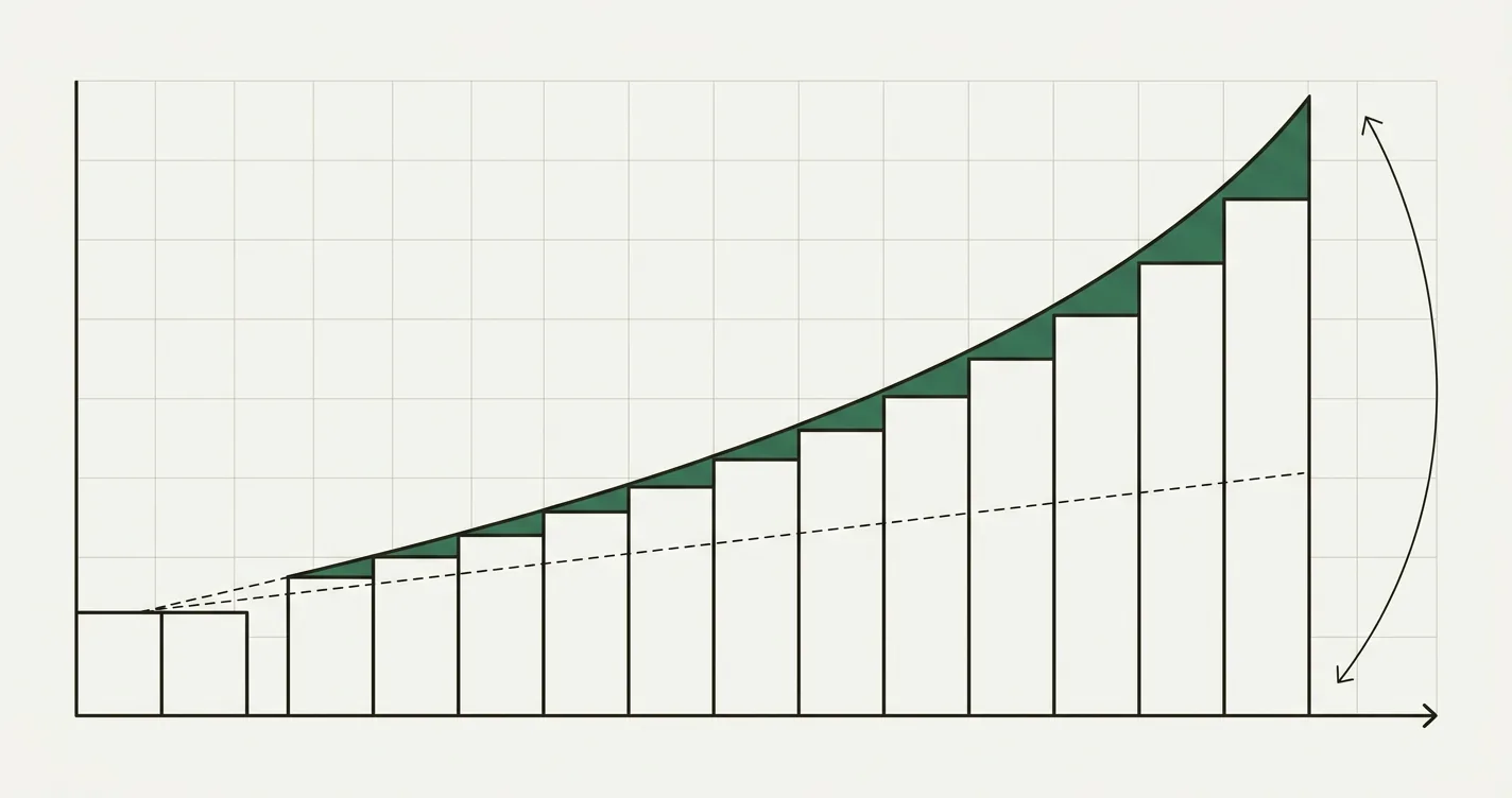
Compound interest is interest earned on interest. Each period, the interest a balance generates is added back to the balance, so the next period's interest is calculated on a slightly larger base. Repeated over many periods, that feedback loop turns a straight line into a curve - and it is the same curve, viewed from the other end, that discounting flattens back to a present value.
Simple interest, by contrast, is charged only on the original principal and grows in a straight line. Almost nothing in finance uses simple interest: loans, deposits, bonds, and every valuation model compound. Getting the compounding mechanics exactly right - the rate, the frequency, the number of periods - is the difference between a model that ties and one that is quietly off by thousands.
Compounding moves a cash flow forward in time; discounting is the identical formula run backward. Both sit at the core of every financial model.
The Compound Interest Formula
The future value of a single sum under compound interest is:
FV = PV x (1 + r / n) ^ (n x t)
Where:
- PV - the present value, or principal: the amount you start with today.
- r - the nominal annual interest rate (the quoted or stated rate), as a decimal.
- n - the number of times interest compounds per year (1 = annual, 12 = monthly, 365 = daily).
- t - the number of years.
- FV - the future value: principal plus all accumulated compound interest.
The compound interest earned on its own is simply FV - PV.
Two terms do all the work. r / n is the periodic rate - the interest rate for one compounding period. n x t is the total number of periods. Everything else is bookkeeping.
Annual compounding
When interest compounds once a year, n = 1 and the formula collapses to the version most people memorise:
FV = PV x (1 + r) ^ t
Simple interest, for contrast
FV = PV x (1 + r x t)
Take $250,000 at 6% for 5 years:
- Simple interest: 250,000 x 0.06 x 5 = $75,000 of interest, for $325,000 total.
- Compound interest (annual): 250,000 x (1.06)^5 = $334,556, so $84,556 of interest.
The $9,556 difference is entirely interest earning interest - and it grows every year the money stays invested.
Continuous compounding
As n grows without limit, (1 + r / n)^(n x t) approaches a clean exponential:
FV = PV x e ^ (r x t)
Continuous compounding is the theoretical ceiling: it produces the highest future value any nominal rate r can reach. It appears in options pricing and academic finance; in a corporate model it is rarely worth the loss of transparency.
Compounding Periods: Why Frequency Matters
Hold the nominal rate fixed at 8% and invest $10,000 for one year. The only thing that changes below is how often interest is added:
| Compounding frequency | Periods/yr (n) | Rate per period (r / n) | Future value | Effective annual rate |
|---|---|---|---|---|
| Annual | 1 | 8.000% | $10,800.00 | 8.000% |
| Semi-annual | 2 | 4.000% | $10,816.00 | 8.160% |
| Quarterly | 4 | 2.000% | $10,824.32 | 8.243% |
| Monthly | 12 | 0.667% | $10,830.00 | 8.300% |
| Daily | 365 | 0.0219% | $10,832.78 | 8.328% |
| Continuous | - | - | $10,832.87 | 8.329% |
Going from annual to monthly compounding adds $30 on $10,000 - real, but small. Going from monthly all the way to continuous adds under $3 more. This is why most corporate models compound annually or monthly and stop there.
The effective annual rate
The right-hand column is the effective annual rate (EAR), also called APY - the rate that, compounded just once a year, gives the same result as the nominal rate compounded n times:
EAR = (1 + r / n) ^ n - 1
The EAR is the only honest way to compare rates with different compounding conventions. A credit line quoted at "12% per year, compounded monthly" has a periodic rate of 1% and an effective annual cost of:
EAR = (1 + 0.12 / 12) ^ 12 - 1 = (1.01) ^ 12 - 1 = 12.683%
So a "12%" card actually costs 12.68% a year. Always convert to an EAR before comparing, and feed the EAR - not the nominal rate - into an annual model.
Worked Example: Growing a Single Sum
Invest $250,000 at a 6% nominal annual rate for 5 years. Start with annual compounding and build the balance one year at a time:
| Year | Opening balance | Interest at 6% | Closing balance |
|---|---|---|---|
| 1 | $250,000.00 | $15,000.00 | $265,000.00 |
| 2 | $265,000.00 | $15,900.00 | $280,900.00 |
| 3 | $280,900.00 | $16,854.00 | $297,754.00 |
| 4 | $297,754.00 | $17,865.24 | $315,619.24 |
| 5 | $315,619.24 | $18,937.15 | $334,556.39 |
Each year's interest is charged on the previous closing balance, which is why the interest column climbs from $15,000 to $18,937 even though the rate never changes. The formula gets there in one step:
FV = 250,000 x (1.06) ^ 5 = $334,556.39
Now change the compounding frequency
Keep the 6% nominal rate and the 5-year horizon; only n changes:
| Compounding | Future value | Compound interest | Gain vs. annual |
|---|---|---|---|
| Annual (n = 1) | $334,556.39 | $84,556.39 | - |
| Quarterly (n = 4) | $336,713.75 | $86,713.75 | +$2,157.36 |
| Monthly (n = 12) | $337,212.54 | $87,212.54 | +$2,656.15 |
| Continuous | $337,464.70 | $87,464.70 | +$2,908.31 |
Monthly compounding beats annual by $2,656.15 over five years on a quarter-million-dollar balance. Continuous adds only $252.16 on top of monthly - the curve of "more frequent compounding" flattens fast.
The monthly figure comes from a 0.5% periodic rate over 60 periods. The first three months and the last:
| Month | Opening balance | Interest at 0.5% | Closing balance |
|---|---|---|---|
| 1 | $250,000.00 | $1,250.00 | $251,250.00 |
| 2 | $251,250.00 | $1,256.25 | $252,506.25 |
| 3 | $252,506.25 | $1,262.53 | $253,768.78 |
| ... | ... | ... | ... |
| 60 | $335,534.87 | $1,677.67 | $337,212.54 |
FV = 250,000 x (1 + 0.06 / 12) ^ (12 x 5) = 250,000 x (1.005) ^ 60 = $337,212.54
Compound Interest in Excel
Three routes, and they must all agree. If they do not, one of them has the rate or the period count wrong.
Method 1 - The caret operator (most transparent)
// Annual: rate in B1, years in B2, principal in B3
= B3 * (1 + B1) ^ B2                 // 250000 * 1.06^5  ->  334556.39

// Sub-annual: divide the rate by n, multiply the periods by n
= B3 * (1 + B1 / 12) ^ (B2 * 12)     // monthly  ->  337212.54
Method 2 - The FV() function
FV(rate, nper, pmt, [pv], [type]). For a lump sum with no recurring payment, pmt is 0 and the present value is entered as a negative number, because paying money in is a cash outflow:
= FV(0.06, 5, 0, -250000)            // annual   ->  334556.39
= FV(0.06/12, 5*12, 0, -250000)      // monthly  ->  337212.54
Method 3 - Nominal and effective rate helpers
= EFFECT(0.06, 12)                   // nominal -> effective:  0.061678  (6.168%)
= NOMINAL(0.061678, 12)              // effective -> nominal:  0.060000

// Continuous compounding
= 250000 * EXP(0.06 * 5)             // 337464.70
The roll-forward, for a model you want to audit
When compounding needs to be visible on the sheet - inside a debt schedule or a savings build - lay out one row per period:
// $B$1 = periodic rate; B2 = opening balance for the period
= B2 * $B$1          // interest for the period
= B2 + C2            // closing balance, which becomes the next row's opening
From Compounding to Discounting
Every valuation model runs the compound interest formula backward. Compounding asks "what is a dollar today worth in the future?" and multiplies by the growth factor. Discounting asks "what is a future dollar worth today?" and divides by the very same factor:
Discount factor for period t = 1 / (1 + r) ^ t
That is the reciprocal of (1 + r)^t. Where compounding takes $250,000 to $334,556 over five years at 6%, discounting takes $334,556 straight back:
PV = 334,556.39 / (1.06) ^ 5 = $250,000.00
Applied to a forecast, the same move turns projected cash flows into a value today. For example, $80,000 of free cash flow in year 3, discounted at a 9% rate:
Discount factor (year 3) = 1 / (1.09) ^ 3 = 1 / 1.295029 = 0.772183
PV = 80,000 / 1.295029 = $61,774.68
Do this for every year of the forecast, add a discounted terminal value for the years beyond it, and sum - that total is the present value of the business, the heart of a discounted cash flow model. The rate r there is the weighted average cost of capital, but the arithmetic of moving money through time is identical to a savings account.
Compounding a Stream: Future Value of an Annuity
A single sum is the simple case. When an equal cash flow arrives every period and each deposit compounds from the date it lands, the future value of that stream is:
FV of an ordinary annuity = C x [ ( (1 + r) ^ n - 1 ) / r ]
Where C is the cash flow per period, r the periodic rate, and n the number of payments. The bracketed term is the future-value annuity factor - the sum of the growth factors for each individual deposit.
Example: deposit $12,000 at the end of each year for 10 years, earning 7% annually:
Annuity factor = ( (1.07) ^ 10 - 1 ) / 0.07 = ( 1.96715136 - 1 ) / 0.07 = 13.816448
FV = 12,000 x 13.816448 = $165,797.38
You contribute $120,000 over the decade; the other $45,797 is compound interest. In Excel, the pmt argument carries the recurring flow:
= FV(0.07, 10, -12000, 0, 0)        // deposits at period end    ->  165797.38
= FV(0.07, 10, -12000, 0, 1)        // deposits at period start   ->  177403.19
Switching type from 0 to 1 moves every deposit one period earlier, so each one compounds for an extra year - worth $11,606 here.
The Rule of 72 and CAGR
Two familiar shortcuts are the compound interest formula in disguise.
The Rule of 72 estimates how long a balance takes to double: divide 72 by the interest rate in percentage points. At 6%, a balance doubles in roughly 72 / 6 = 12 years; solving the formula exactly gives ln(2) / ln(1.06) = 11.9 years. At 8% the rule says 9 years against an exact 9.01. The approximation holds for rates between about 4% and 12%.
CAGR (compound annual growth rate) is the formula rearranged to solve for the rate instead of the future value:
CAGR = (Ending value / Beginning value) ^ (1 / t) - 1
If a figure grows from $250,000 to $334,556 over 5 years, CAGR = (334,556 / 250,000) ^ (1/5) - 1 = 6.00% - recovering the rate the growth was built from. See CAGR: how to calculate compound annual growth rate for the full treatment, including where it misleads.
Common Mistakes to Avoid
- Mixing the rate and the period. A 6% annual rate in a monthly model must become 0.5% per month over 60 periods - not 6% over 60. Feeding an annual rate into a monthly schedule overstates growth wildly.
- Comparing nominal rates with different compounding. 5.9% compounded monthly (6.06% EAR) beats 6.0% compounded annually. Convert everything to an effective annual rate first.
- Sign and argument errors in FV(). Excel's
FV()treatspvas today's balance andpmtas a recurring flow. Swapping them, or forgetting that outflows are negative, silently corrupts the answer. - Off-by-one on the period count. Five years of annual compounding is an exponent of 5. Count the gaps between dates, not the dates themselves.
- Compounding something that should not compound. Percentages that describe a ratio - margins, tax rates, growth-on-growth assumptions - do not carry a balance forward. Only quantities with a balance (money, units, an index level) compound.
- Defaulting to simple interest. Unless a contract explicitly specifies it, multi-period interest compounds. Simple interest understates every balance past year one, and the gap widens over time.
- Over-precising the frequency. Past monthly, the extra future value from daily or continuous compounding is a rounding error on most models - a few dollars on a quarter-million over five years. Do not let it drive a decision.

Alex Tapio
Founder of Finamodel • Professional Financial Modeller • Ex-Deloitte