LBO Returns Bridge: What Drives Private Equity Returns

Key Takeaways
- The bridge has three levers - EBITDA growth, multiple change, and debt paydown - and they sum exactly to exit equity minus entry equity when you value EBITDA growth at the entry multiple and the multiple change on exit EBITDA.
- EBITDA growth is the lever a sponsor controls, and it dominates a healthy return profile. In the worked example it is 64% of value created; strip it out and a 27% IRR collapses to 12%.
- Debt paydown converts operating cash into equity dollar for dollar. Higher entry leverage and faster cash conversion amplify it - here it is 27% of value created and 3.8 turns of deleveraging.
- Multiple expansion is a market gift, not a plan. Underwrite flat-to-down; in the example a half-turn of expansion is under 9% of value created and about 1.5 points of IRR.
- Always carry a check row. The three components minus the change in equity value must equal zero.
- Convert the bridge to MOIC contributions by dividing each piece by entry equity - those are additive and slide-ready - then run a two-way sensitivity on exit multiple and exit EBITDA to see which cells still clear your hurdle.
- Use XIRR on dated cash flows whenever there is a dividend recap or a non-annual hold; the simple annualised-multiple formula only holds for one cash outflow and one inflow.
For the full build behind these numbers, see the LBO model tutorial, the paper LBO walk-through, and the debt schedule guide. To pressure-test the entry EBITDA you are paying for, read quality of earnings adjustments, and to build the model itself, start from the LBO model template.
An LBO returns bridge decomposes the equity value a private equity sponsor creates into three levers: EBITDA growth, change in the valuation multiple, and debt paydown. Get the conventions right and the three components sum exactly to exit equity value minus entry equity value, turning the bridge into both a model check and the story you tell an investment committee. This guide builds one from scratch with a full worked example, the Excel formulas, an IRR attribution, and a two-way sensitivity table.
Every leveraged buyout makes money in a small number of ways, and a returns bridge is the exhibit that names them. It answers the question a limited partner actually asks: of the 3x we returned, how much came from running the business better, how much from paying down debt with its cash flow, and how much from simply selling into a friendlier market than the one we bought in?
That distinction matters because the three levers are not equally repeatable. EBITDA growth is the one a sponsor controls through the operating plan. Debt paydown is mechanical once the capital structure and cash conversion are set. Multiple expansion is a market gift that a disciplined underwriter never counts on. A bridge that shows most of the value coming from operations is a very different diligence signal than one that leans on the exit multiple.
The LBO returns bridge: three levers that convert entry equity into exit equity.
What the bridge decomposes
Start from the two anchor points. At entry, the sponsor writes an equity check equal to purchase enterprise value less the debt raised:
Entry Equity = Entry EBITDA x Entry Multiple - Entry Net Debt
At exit, the equity is whatever the business is worth less the debt still outstanding:
Exit Equity = Exit EBITDA x Exit Multiple - Exit Net Debt
The total value the sponsor created is Exit Equity - Entry Equity. The bridge splits that single number into three pieces:
- EBITDA growth - the extra earnings generated over the hold, valued at the multiple you paid:
(Exit EBITDA - Entry EBITDA) x Entry Multiple. - Multiple change - the re-rating (or de-rating) of the business, applied to exit earnings:
(Exit Multiple - Entry Multiple) x Exit EBITDA. - Debt paydown - the reduction in net debt over the hold, funded by cumulative free cash flow:
Entry Net Debt - Exit Net Debt.
The reason the multiple change is applied to exit EBITDA while EBITDA growth is valued at the entry multiple is not arbitrary. Expand the two expressions and the shared terms cancel, leaving exactly Exit EBITDA x Exit Multiple - Entry EBITDA x Entry Multiple, which is the change in enterprise value with no leftover interaction term. Add the change in net debt and you have the change in equity value. The bridge closes by construction. If you build it any other way, keep a check row and watch it fail.
This walk-through assumes you already have a working buyout model. If you need the underlying mechanics first, see the LBO model tutorial and the debt schedule guide.
The formulas in Excel
Put every input on an assumptions sheet as a named range and let the bridge reference them:
// Entry: enterprise value and sponsor equity
= Entry_EBITDA * Entry_Multiple                       // Entry enterprise value
= Entry_EV - Entry_NetDebt                            // Entry equity (sponsor cash in)

// Exit: enterprise value and equity at end of hold
= Exit_EBITDA * Exit_Multiple                         // Exit enterprise value
= Exit_EV - Exit_NetDebt                              // Exit equity value

// The three bridge components
= (Exit_EBITDA - Entry_EBITDA) * Entry_Multiple       // 1. EBITDA growth
= (Exit_Multiple - Entry_Multiple) * Exit_EBITDA      // 2. Multiple change
= Entry_NetDebt - Exit_NetDebt                        // 3. Debt paydown

// Check row - must equal exactly zero
= EBITDA_Growth + Multiple_Change + Debt_Paydown - (Exit_Equity - Entry_Equity)
The check row is not optional. It is the single fastest way to catch a sign error in net debt, a stray reference to the wrong multiple, or a hardcoded number that should have been a formula.
Worked example: the setup
We buy a business at the start of Year 0 and sell it at the end of Year 5. The entry is a 10.0x EV/EBITDA purchase financed 60/40 debt to equity, so net debt at close is 6.0x EBITDA. Over the hold, revenue compounds at roughly 5% a year and the EBITDA margin improves from 20.0% to 25.0%, lifting EBITDA from $100.0M to $160.0M (a 9.9% EBITDA CAGR). We underwrite a modest half-turn of multiple expansion to 10.5x.
| Assumption | At entry (Year 0) | At exit (Year 5) |
|---|---|---|
| Revenue | $500.0M | $640.0M |
| EBITDA margin | 20.0% | 25.0% |
| EBITDA | $100.0M | $160.0M |
| EV / EBITDA multiple | 10.0x | 10.5x |
| Enterprise value | $1,000.0M | $1,680.0M |
| Net debt | $600.0M | $345.9M |
| Net debt / EBITDA | 6.0x | 2.2x |
| Equity value | $400.0M | $1,334.1M |
Entry equity is $1,000.0M - $600.0M = $400.0M. Exit equity is $1,680.0M - $345.9M = $1,334.1M. The exit net debt figure comes from the debt schedule below.
Building the debt paydown line
Debt paydown in the bridge is just the cumulative free cash flow the business swept against its net debt over five years. Model it as EBITDA less cash interest on the opening balance, less capex and the change in working capital, less cash taxes. Every dollar of that free cash flow reduces net debt and therefore lands in equity at exit.
| ($M) | Year 1 | Year 2 | Year 3 | Year 4 | Year 5 |
|---|---|---|---|---|---|
| EBITDA | 111.0 | 123.0 | 136.0 | 148.0 | 160.0 |
| Cash interest (8% of opening net debt) | (48.0) | (45.8) | (42.7) | (38.7) | (33.7) |
| Capex + change in NWC | (24.0) | (26.0) | (28.0) | (30.0) | (32.0) |
| Cash taxes | (11.0) | (13.0) | (15.0) | (17.0) | (19.0) |
| Free cash flow for debt paydown | 28.0 | 38.2 | 50.3 | 62.3 | 75.3 |
| Opening net debt | 600.0 | 572.0 | 533.8 | 483.5 | 421.2 |
| Closing net debt | 572.0 | 533.8 | 483.5 | 421.2 | 345.9 |
// Cash interest on the opening balance
= OpeningNetDebt * Cash_Interest_Rate

// Free cash flow available to sweep against debt
= EBITDA - Cash_Interest - Capex - Change_in_NWC - Cash_Taxes

// Closing net debt after the sweep
= OpeningNetDebt - FCF_for_Debt_Paydown

// Cumulative paydown over the hold (feeds the bridge)
= Entry_NetDebt - Closing_NetDebt_Year5
Cumulative free cash flow is 28.0 + 38.2 + 50.3 + 62.3 + 75.3 = $254.1M. Net debt falls from $600.0M to $600.0M - $254.1M = $345.9M, a swing of 3.8 turns of leverage (6.0x down to 2.2x). That $254.1M is the debt paydown component of the bridge.
Assembling the bridge
Now drop the three components in. EBITDA grew by $60.0M, valued at the 10.0x entry multiple. The multiple rose half a turn, applied to $160.0M of exit EBITDA. Net debt fell by $254.1M.
| Value driver | Calculation | Contribution ($M) | Share of value created | MOIC contribution |
|---|---|---|---|---|
| Entry equity (returned at exit) | - | - | - | 1.00x |
| EBITDA growth | $60.0M x 10.0x | 600.0 | 64.2% | 1.50x |
| Multiple expansion | +0.5x x $160.0M | 80.0 | 8.6% | 0.20x |
| Debt paydown | cumulative FCF sweep | 254.1 | 27.2% | 0.64x |
| Total value created | 934.1 | 100.0% | +2.34x | |
| Exit equity value | 1,334.1 | 3.34x |
Check: 600.0 + 80.0 + 254.1 = 934.1, and $1,334.1M - $400.0M = $934.1M. The bridge ties.
The MOIC contribution column is each dollar figure divided by the $400.0M entry equity check. Because that denominator is constant, the pieces are additive: 1.00 + 1.50 + 0.20 + 0.64 = 3.34x. This is the version of the bridge you put on a slide, because it reads directly as "we turned 1.0x into 3.3x, and here is where each 0.x came from."
The story this particular deal tells: operating improvement did roughly two thirds of the work, using its own cash to deleverage did about a quarter, and the market re-rating chipped in under a tenth. That is a healthy profile. A bridge where those weights are reversed is one an investment committee should push on hard.
From value creation to MOIC and IRR
The money multiple falls straight out of the bridge:
MOIC = Exit Equity / Entry Equity = $1,334.1M / $400.0M = 3.34x
With a single equity outflow at close and a single inflow at exit, the IRR is just the multiple annualised over the hold:
IRR = MOIC ^ (1 / Hold Years) - 1 = 3.34 ^ (1 / 5) - 1 = 27.2%
// Money multiple
= Exit_Equity / Entry_Equity

// Annualised IRR for a single entry and single exit
= (Exit_Equity / Entry_Equity) ^ (1 / Hold_Years) - 1

// IRR with a dividend recap or a non-annual hold - use dated cash flows
= XIRR(equity_cash_flows, cash_flow_dates)
If the deal includes a dividend recapitalisation partway through the hold, do not force it into the simple formula. List the dated equity cash flows (negative at close, positive on the recap date, positive at exit) and use XIRR. The recap still shows up in the bridge as part of debt paydown running in reverse, netted against distributions received. For the difference between the time-blind multiple and the time-weighted rate, see IRR vs MOIC.
Splitting EBITDA growth into revenue and margin
The single largest bar in most bridges is EBITDA growth, so it is worth breaking down one level further. Hold the margin flat and let only revenue grow to isolate the volume effect; then apply the margin gain to exit revenue to isolate the efficiency effect.
| Component | Calculation | EBITDA effect | EV effect at 10.0x |
|---|---|---|---|
| Revenue growth (margin held at 20.0%) | $640.0M x 20.0% - $100.0M | +$28.0M | +$280.0M |
| Margin expansion (on exit revenue) | $640.0M x (25.0% - 20.0%) | +$32.0M | +$320.0M |
| Total EBITDA growth | +$60.0M | +$600.0M |
Here the split is roughly even: $28.0M + $32.0M = $60.0M, worth $280.0M + $320.0M = $600.0M of enterprise value at the entry multiple. In diligence this matters because 500 basis points of margin expansion is a very different underwriting claim than 5% annual revenue growth. One depends on a cost programme the sponsor can name; the other depends on the market.
IRR attribution: switching one lever off at a time
MOIC attribution is additive. IRR attribution is not, because the rate compounds and the levers interact through the capital structure (more leverage means more interest, which means less free cash flow for paydown). The workable method is to re-run the model with one lever neutralised and report the IRR it produces. Hold everything else at base case.
| Scenario | Exit equity ($M) | MOIC | 5-year IRR |
|---|---|---|---|
| Full deal (base case) | 1,334.1 | 3.34x | 27.2% |
| No multiple expansion (exit at 10.0x) | 1,254.1 | 3.14x | 25.7% |
| No EBITDA growth (EBITDA flat at $100.0M, exit 10.5x) | 704.1 | 1.76x | 12.0% |
| No leverage (all-equity, $1,000.0M invested) | 1,680.0 | 1.68x | 10.9% |
Read these as sensitivities, not as a partition: the deltas do not sum to the base-case IRR, and the no-leverage row in particular is illustrative because an all-equity deal would also throw off more distributable cash during the hold. Still, the ranking is stark. Strip out EBITDA growth and a 27% deal becomes a 12% deal. Strip out leverage and it roughly halves. Strip out the half-turn of multiple expansion and you lose about 1.5 points. That ordering is the whole argument for underwriting operating improvement rather than financial engineering.
Sensitivity: exit multiple against exit EBITDA
The two assumptions the bridge is most exposed to are the exit multiple and the level of exit EBITDA. Build a two-way table of equity IRR across both, holding exit net debt at $345.9M and the hold at five years.
| Exit multiple \ Exit EBITDA | $140M | $150M | $160M | $170M | $180M |
|---|---|---|---|---|---|
| 9.0x | 18.0% | 20.2% | 22.3% | 24.2% | 26.1% |
| 9.5x | 19.7% | 22.0% | 24.0% | 26.0% | 27.8% |
| 10.0x | 21.4% | 23.6% | 25.7% | 27.6% | 29.5% |
| 10.5x | 23.0% | 25.2% | 27.2% | 29.2% | 31.0% |
| 11.0x | 24.5% | 26.7% | 28.7% | 30.7% | 32.5% |
The base case sits at the 10.5x / $160M intersection at 27.2%. The instructive part is the bottom-left quadrant: even with the multiple contracting a full turn to 9.0x, as long as EBITDA still reaches $160M the deal returns 22.3%. The operating plan carries the return. A fund with a 20% gross IRR hurdle clears it in every cell of this grid except the two worst corners, which tells you the underwriting has a real margin of safety in EBITDA even if the exit environment disappoints.
Common mistakes to avoid
- Mixing the multiple conventions. Valuing EBITDA growth at the exit multiple and the multiple change on entry EBITDA double-counts the interaction term. Fix the convention: change-in-EBITDA at the entry multiple, change-in-multiple on exit EBITDA. Then the bridge ties.
- No check row. Always carry
components - (exit equity - entry equity)and confirm it is zero. It is the only line that catches a net-debt sign error or a wrong cell reference before the memo goes out. - Underwriting multiple expansion as base case. Assume the exit multiple is flat or slightly below entry. Treat any expansion as upside you did not pay for, not as a pillar of the thesis.
- Confusing EBITDA growth with revenue growth. Margin expansion is a separate lever with a separate diligence burden. Split the EBITDA growth bar into a volume piece and a margin piece.
- Ignoring transaction fees, management equity, and rollover. The bridge should reconcile to the sponsor's net cash in and out. Financing fees and the management option pool sit between gross equity value and the sponsor's proceeds.
- Using simple CAGR IRR when cash flows are irregular. A dividend recap or a delayed close breaks the single-in, single-out assumption. Use
XIRRon dated cash flows. - Net debt sign errors. Cash nets against debt. A build in the cash balance during the hold reduces net debt and helps equity; a working-capital release does the same. Get the direction right or the paydown line will be backwards.
- Treating a dividend recap as a fourth independent lever. It is not. A recap adds debt back, so it shows up as negative debt paydown, offset by the distribution the sponsor receives. Double-counting it inflates the bridge.

Alex Tapio
Founder of Finamodel • Professional Financial Modeller • Ex-Deloitte